Middle to Late Holocene Variations in Salinity and Primary Productivity in the Central Baltic Sea: A Multiproxy Study From the Landsort Deep
 Falkje van Wirdum1*
  Elinor Andrén1
  Denise Wienholz2
  Ulrich Kotthoff2,3
  Matthias Moros4
  Anne-Sophie Fanget5
  Marit-Solveig Seidenkrantz6,7
  Thomas Andrén1
- 1School of Natural Sciences, Technology and Environmental Studies, Södertörn University, Huddinge, Sweden
- 2Institute for Geology, University of Hamburg, Hamburg, Germany
- 3Center of Natural History, University of Hamburg, Hamburg, Germany
- 4Leibniz Institute for Baltic Sea Research Warnemünde, Rostock, Germany
- 5CEFREM, University of Perpignan, Perpignan, France
- 6Centre for Past Climate Studies, Department of Geoscience, Aarhus University, Aarhus, Denmark
- 7iCLIMATE Aarhus University Interdisciplinary Centre for Climate Change, Aarhus, Denmark
Anthropogenic forcing has led to an increased extent of hypoxic bottom areas in the Baltic Sea during recent decades. The Baltic Sea ecosystem is naturally prone to the development of hypoxic conditions due to its geographical, hydrographical, geological, and climate features. Besides the current spreading of hypoxia, the Baltic Sea has experienced two extensive periods of hypoxic conditions during the Holocene, caused by changing climate conditions during the Holocene Thermal Maximum (HTM; 8–4.8 cal ka BP) and the Medieval Climate Anomaly (MCA; 1–0.7 cal ka BP). We studied the variations in surface and bottom water salinity and primary productivity and their relative importance for the development and termination of hypoxia by using microfossil and geochemical data from a sediment core retrieved from the Landsort Deep during IODP Expedition 347 (Site M0063). Our findings demonstrate that increased salinity was of major importance for the development of hypoxic conditions during the HTM. In contrast, we could not clearly relate the termination of this hypoxic period to salinity changes. The reconstructed high primary productivity associated with the hypoxic period during the MCA is not accompanied by considerable increases in salinity. Our proxies for salinity show a decreasing trend before, during and after the MCA. Therefore, we suggest that this period of hypoxia is primarily driven by increasing temperatures due to the warmer climate. These results highlight the importance of natural climate driven changes in salinity and primary productivity for the development of hypoxia during a warming climate.
Introduction
Oxygen concentrations have been declining worldwide in both the open oceans and coastal waters since the mid-20th century (Breitburg et al., 2018). Hypoxia (<2 mg/l dissolved oxygen) has become common in coastal seas, deteriorating ecosystem structure and functioning (Zhang et al., 2010). This spreading of hypoxia during recent decades has been associated with human activities and global climate warming (Diaz and Rosenberg, 2008). Hypoxia is a severe environmental problem in the Baltic Sea (Figure 1), where over 20% of all known coastal hypoxic sites are located (Conley et al., 2011). This marginal sea is considered a key area for studying the factors governing hypoxia (Carstensen et al., 2014).
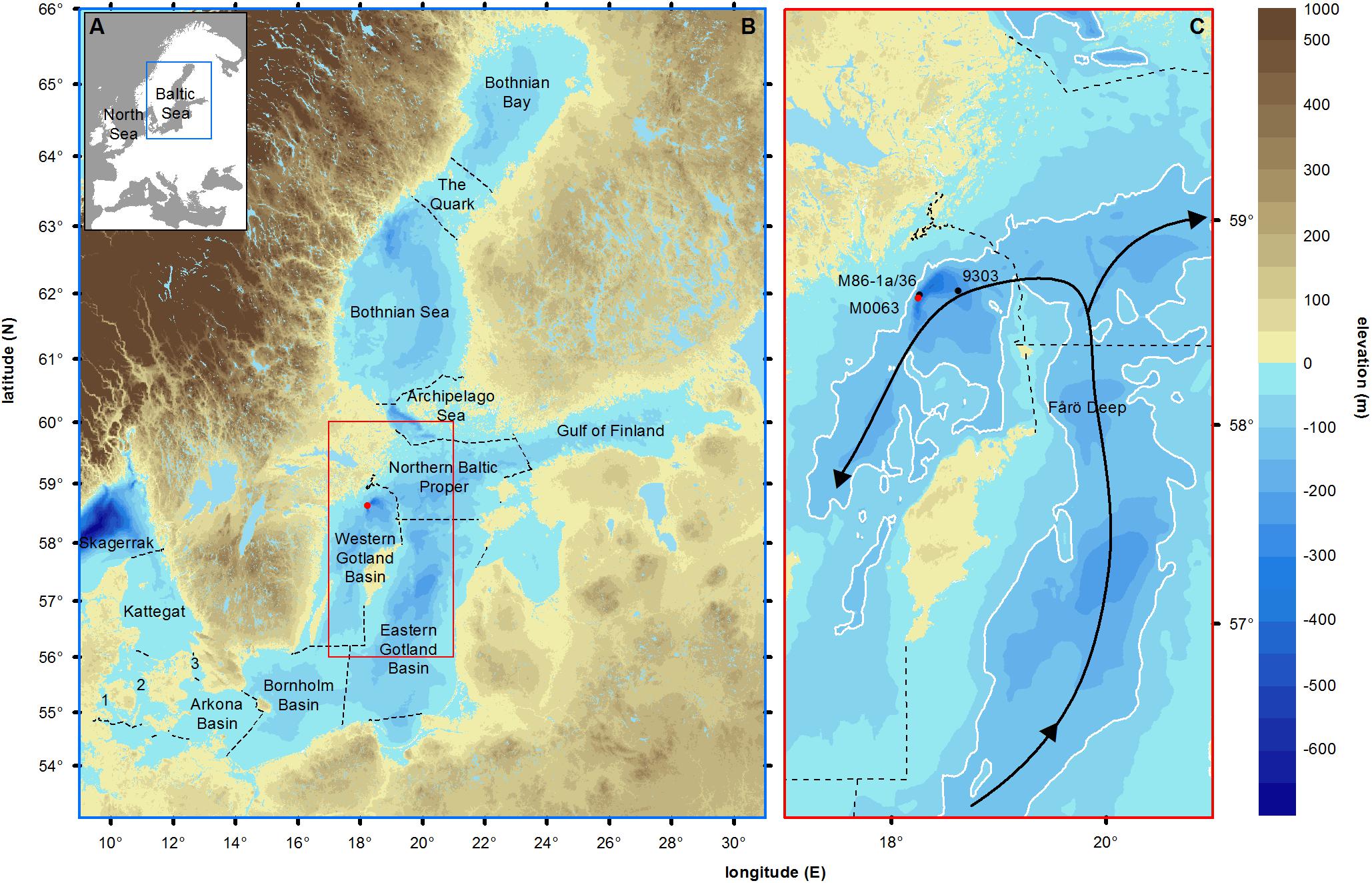
Figure 1. (A) Map of Europe showing the semi-enclosed position of the Baltic Sea. (B) Land elevation (brown shades, meters), bathymetry (blue shades, meters) and main sub-basins of the Baltic Sea (dotted lines, according to HELCOM). Skagerrak and Kattegat form the transition zone to the North Sea. The Little Belt (1), Great Belt (2), and Öresund (3) form the connections to the North Sea. The Arkona Basin, Bornholm Basin, Eastern Gotland Basin, Northern Baltic Proper and Western Gotland Basin form the Baltic Proper. The Bothnian Sea, The Quark and the Bothnian Bay form the Gulf of Bothnia. (C) Inset of the studied area. The red dot represents the studied Integrated Ocean Drilling Program Expedition 347 site M0063 (Landsort Deep, 58°37.350’N, 18°15.260’E, Andrén et al., 2015). The black dots represent the sites 435-2 (Warden et al., 2017) and 9303 (Bianchi et al., 2000), used for comparison of carbon data and corresponding ages to data of core M0063D. White lines indicate 100 m depth contours. Black arrows show the directions of inflowing deep-water. Geospatial data are provided by HELCOMs Map and Database Service (http://maps.helcom.fi).
The Baltic Sea is a semi-enclosed brackish sea connected to the North Sea through the Little and Great Belts and the Öresund (Figure 1). With a mean depth of 54 m and an area of 393,000 km2 (Leppäranta and Myrberg, 2009), its basin is overall relatively small and shallow. The deepest sub-basin is the Landsort Deep (459 m, Figure 1). Natural climate forcing regulates the water exchange between the North Sea and the Baltic Sea, which is of high importance for the environmental conditions throughout the basin (Elken and Matthäus, 2008). Inflows from the North Sea affect the salt and oxygen concentrations in the deep waters (Mohrholz et al., 2015). Stronger salinity stratification and increased primary productivity have been identified as two important climatic forcing factors in driving hypoxia before intense human impact (Papadomanolaki et al., 2018), yet their relative importance is not fully understood (Zillén et al., 2008; Schimanke et al., 2012; Jokinen et al., 2018). Nine coastal countries surround the Baltic Sea and over 85 million people inhabit its drainage basin. At present, anthropogenic forcing exerts a wide variety of pressures on the Baltic Sea ecosystem (Helcom, 2017). A major threat to the ecosystem is eutrophication, caused by excessive input of nutrients to the sea (Andersen et al., 2017). This has a positive feedback on the spreading of hypoxic zones (Zillén and Conley, 2010). Both natural and human-induced changes of the Baltic Sea ecosystem play a role in the current spreading of hypoxic zones (Zillén and Conley, 2010; Meier et al., 2017), but their relative importance is difficult to separate.
We aim to establish the natural variability in environmental conditions in the Baltic Proper (Figure 1) during the middle and late Holocene (respectively, 8.2 – 4.2 cal ka BP and 4.2 ka BP - present; Walker et al., 2012) using a multiproxy approach. We focus on reconstructing variability in salinity and primary productivity and establishing their roles in driving redox conditions in the Landsort Deep (Figure 1). Variations in the assemblage and concentrations of fossil diatoms, silicoflagellates, dinoflagellate cysts (hereafter dinocysts), and Radiosperma corbiferum (hereafter Radiosperma) reflect changes in surface water salinity. In contrast, benthic foraminiferal concentrations reflect variations in bottom water salinity and oxygenation and can thus pinpoint intrusions of well-oxygenated saline water to the sea floor. Lithological characteristics of sediments allow for interpretations of redox conditions at the sediment-water interface. Diatom concentration and biogenic silica content of the sediments provide information on changes in diatom production. The total carbon content of the sediments represents changes in gross primary production. Relative pollen abundances are applied as indicators of terrestrial ecosystem and climate change.
This study provides information needed for assessing the consequences of ongoing and future changes in salinity and primary productivity for the Baltic Sea ecosystem. Ongoing anthropogenic and natural climate forcing on the Baltic Sea ecosystem are expected to increase primary productivity (Meier et al., 2011b, 2012; Storch von et al., 2015). Whether, the salinity of the Baltic Sea will increase or decrease is uncertain (Meier et al., 2011a, 2017). Assessing the impact of such changes on redox conditions in the water column can be projected to present and future changes in the Baltic Sea ecosystem and used to design action plans to improve its status by adjusting human actions.
Regional Setting
Present Baltic Sea
The salt balance of the Baltic Sea is governed by evaporation (Leppäranta and Myrberg, 2009); freshwater input from rivers and precipitation (Bergstrom and Carlsson, 1994); and saline inflows from the North Sea (Mohrholz et al., 2015), which maintain the brackish character of the basin. Such inflows are forced either by wind and differences in air pressure (Matthäus, 2006) or by the salinity gradient between the Baltic Sea and Kattegat (Figure 1; Mohrholz et al., 2006). In the Baltic Proper (Figure 1) surface water salinity is on average 7 and bottom water salinities vary between 11 and 13 (Mohrholz et al., 2015). This vertical salinity gradient results in the presence of a permanent halocline (at c. 60 m water depth), which isolates bottom waters from surface waters. Therefore, ventilation of the deeper waters strongly depends on marine inflows (Figure 1C).
Only episodic large inflows of highly saline and oxygenated water can renew the deep waters in the Baltic Proper (Matthäus et al., 2008). These events, known as major Baltic inflows, occur mainly during winter and depend on the prevailing wind-regime (Matthäus, 2006; Mohrholz et al., 2015). Although these inflows bring in oxygen to the deep waters, they also cause increased stability of stratification. This results in stagnation of the bottom waters for several years (Matthäus et al., 2008). Therefore, marine inflows do not necessarily lead to improved oxygen conditions and can actually result in an expansion of hypoxic areas (Conley et al., 2002; Meier et al., 2017; Neumann et al., 2017).
During periods of high primary productivity organic matter sinks into the stratified deeper waters, where it is decomposed. The limited bottom water ventilation does not replenish the bottom waters with sufficient oxygen to compensate for the oxygen consumed during organic matter degradation (Reissmann et al., 2009). Anoxic bottom conditions lead to regeneration and enrichment of phosphorous in the bottom waters (Jilbert et al., 2011), which alters the ratio of phosphorous to nitrogen available for primary producers. The limiting nutrient for phytoplankton production during spring in the Baltic Proper is nitrogen (Granéli et al., 1990; Lignell et al., 2003; Tamminen and Andersen, 2007; Walve and Larsson, 2010). After the spring phytoplankton bloom, surface waters become nitrogen depleted. During summer, the excess phosphate available leads to potentially harmful blooms of nitrogen-fixing bacteria, which fertilize the sea with nitrogen (Kononen, 2001; Vahtera et al., 2007; Funkey et al., 2014).
Historical Hypoxia in the Baltic Sea
The Baltic Sea has experienced periods of hypoxia before the most recent expansion, which allows the study of driving mechanisms for hypoxic conditions in the past. During the past 16,000 years, the Baltic Sea basin has undergone several brackish and freshwater phases, due to the interplay of the gradual melting of the Scandinavian Ice Sheet, subsequent glacio-isostatic uplift, and changes in eustatic sea level (Björck, 1995; Andrén et al., 2011; Rosentau et al., 2017). These natural climate-driven processes led to variations in water exchange with the North Sea, which in turn led to variations in salinity, aquatic productivity, and oxygen conditions in the Baltic basin. In addition to the current hypoxic period, two distinct intervals of hypoxia during the last c. 8000 years are recorded in the sediments of the Baltic Sea (Zillén et al., 2008). Past periods of hypoxia can be recognized in sediment cores as laminated deposits (Jonsson et al., 1990). These laminations show a distinct pattern of seasonal sediment layers, undisturbed by bottom dwelling organisms.
Hypoxia Between c. 8–4 ka BP
The first period of hypoxia has been dated to c. 8–4 cal ka BP (Zillén et al., 2008). This period coincided with the Holocene Thermal Maximum (HTM, c. 8–4.8 cal ka BP, Seppä et al., 2015). During the HTM, a stable, warm, and dry climate prevailed in northern Europe (Seppä et al., 2009; Renssen et al., 2012; Borzenkova et al., 2015). Maximum salinities were reached in the Baltic Sea during the HTM (Gustafsson and Westman, 2002; Emeis et al., 2003). Combined effects of isostatic rebound and eustatic sea level rise led to increased sill depths of the Baltic basin (Andrén et al., 2011) promoting the inflow of saline waters from the North Sea. The dry conditions during the HTM reduced freshwater discharge to the basin which led to higher salt concentrations (Gustafsson and Westman, 2002; Snowball et al., 2004).
Though marine inflows supplied the bottom waters with oxygen, a halocline developed at the same time and stratified the water column (Carstensen et al., 2014). This stratification led to the development of hypoxic conditions at the sea floor. A subsequent increased bioavailability of phosphorus regenerated from sediments augmented primary productivity at the sea surface, and in turn amplified hypoxic conditions (Sohlenius et al., 2001; Jilbert and Slomp, 2013). After the HTM, land uplift exceeded eustatic sea level rise, and shallowing of the sills resulted in a gradual decrease in salinity (Andrén et al., 2011). The termination of this period of hypoxia has been associated with climate cooling and reduced salinity and subsequent reduced water-column stratification (Carstensen et al., 2014).
Hypoxia Between c. 2–0.8 ka BP
The second period of hypoxia is recorded in the Baltic proper between 2 and 0.8 ka BP (Zillén et al., 2008), partly coinciding with the Roman Warm Period and the Medieval Climate Anomaly (MCA). Pollen-inferred temperature reconstructions from Northern Europe (Seppä et al., 2009) show a warm climate anomaly between c. 3 and 1 ka BP. Temperature peaks around c. 2 ka BP, likely reflecting the Roman Warm Period (c. 2.5–1.6 ka BP; Mann, 2007). The MCA (c. 1–0.7 ka BP; Mann et al., 2009) is observed as a pronounced warm period in multiproxy databases, albeit not as warm as present-day (Mann et al., 2008, 2009). Salinity reconstructions for the Baltic Sea hitherto show no agreement during this hypoxic period. Emeis et al. (2003) show a steady increase in salinity that commenced c. 3 ka BP, whereas Gustafsson and Westman (2002) show that a steady decrease started c. 2 ka BP. Whether salinity played a role in the development of past hypoxic periods is unknown (Meier et al., 2017).
A positive correlation between sea surface temperature and both organic carbon and hypoxia in the Eastern Gotland Basin has been found by Kabel et al. (2012). The increase in organic carbon is partly explained by the surface water temperatures being warm enough for massive cyanobacteria blooms (Kabel et al., 2012). In addition, increased biogenic silica suggests that diatom productivity contributed to the increase in organic carbon as well. Increased primary production leads to increased oxygen consumption in bottom waters and thereby contributed to the development of hypoxic conditions. Kabel et al. (2012) link the spread of hypoxia during this period to increased surface water temperatures, influencing deep-water oxygenation through increased primary productivity. A model based on pollen-records from Sweden suggests that land-use intensified between c. 1–0.5 ka BP. This has been related to an expansion of the population during the MCA in the Baltic Sea drainage area (Åkesson et al., 2015). Therefore, it has been suggested that human-induced eutrophication may have played a role in sustaining hypoxic conditions in the Baltic Sea (Zillén et al., 2008; Zillén and Conley, 2010).
Oxic conditions recorded between c.750 and 50 years BP, coincide with a general cooling climate trend, with coldest conditions during the Little Ice Age (LIA; 550–250 yr BP; Mann et al., 2009). The record of Kabel et al. (2012) shows a decline in organic carbon during the LIA, which is associated to decreased sea surface temperatures, unfavorable for cyanobacteria. This oxic period also covers a period of a decline in the human population in the Baltic Sea region, due to the Black Death (600–400 years BP; Lagerås, 2007). It is debated whether this population decline led to decreased anthropogenic forcing on the Baltic Sea ecosystem, allowing for the return of oxic conditions (Zillén et al., 2008). Noticeably, the roles of salinity, primary productivity and eutrophication in the development of hypoxic conditions between c. 2 and 0.8 ka BP and in the return to oxic conditions have not yet been resolved.
Study Site
Landsort Deep, which reaches a maximum water depth of 459 m, is located in the Western Gotland Basin (Figure 1), along a fault line that has been deepened by glacial erosion (Flodén and Brännström, 1965). The trench is relatively narrow, with a sill depth of 138 m (Lepland and Stevens, 1998). Today, a permanent halocline exists around 50–80 m water depth, which prevents mixing of surface and bottom waters. This is also illustrated by the vertical salinity gradient: surface water salinity in the Landsort Deep is on average 7, while the salinity in the deepest part of the basin is on average 11 (Viktorsson, 2018). Due to minimal vertical mixing, Landsort Deep depends on major Baltic inflows for deep-water renewal. The geography and geometry (i.e., a cleft shaped with very steep walls) of Landsort Deep make it function as a depocenter where post-glacial mud accumulates. The high sedimentation rate in this basin has resulted in a 30 m thick sediment archive for the past c. 8000 years.
Materials and Methods
Material
During the Integrated Ocean Drilling Program (IODP) Expedition 347 in 2013 onboard the R/V Greatship Manisha, sediment cores were recovered from five holes at site M0063 in the central part of Landsort Deep (Figure 1; Andrén et al., 2015). Seismic profiles have been acquired to select the most suitable drilling target for obtaining the longest undisturbed post-glacial sequence (Supplementary Figure S1, Andrén et al., 2015). The results presented in this study are based on analyses on sediment samples from Hole D (58°37.350′N, 18°15.260′E), which was cored using a hydraulic piston corer at a water depth of 437.1 m. Hole D was drilled to a total depth of 86.8 m below seafloor (mbsf). In this study, we focus on sediments from the upper 30 mbsf, which encompass the Mid and Late Holocene.
Adjustment of the Depth Scale
Due to the organic-rich sediments at site M0063, the dissolved methane-gas content in the sediments was considerably high. As gas was released during the recovery process, the cores experienced expansion, resulting in extensive sediment loss at the first hole. Therefore, subsequent holes were cored using an adjusted coring strategy, where only 2 m of sediments was drilled in 3.3 m liners, allowing for expansion of sediments without losing sediments (Andrén et al., 2015). Due to this adjusted coring method, the initial meters below seafloor (mbsf) depth scale had to be adjusted to get a best estimate of initial sediment position at the time of coring, prior to recovery and decompression. Based on the mean gamma density profiles of cores from Hole D, Obrochta et al. (2017) obtained an expansion function that was used to develop a new depth scale, expressed as “adjusted meters below seafloor” (ambsf), including quantification of uncertainty.
Lithostratigraphy
Based on Hole D, the sediment record of site M0063 was divided into seven lithostratigraphic units, covering the Late Glacial and Holocene (Andrén et al., 2015). Here, sediment samples from Unit 1 (Subunits a–d) and Subunits 2a,b have been investigated (Figure 2).
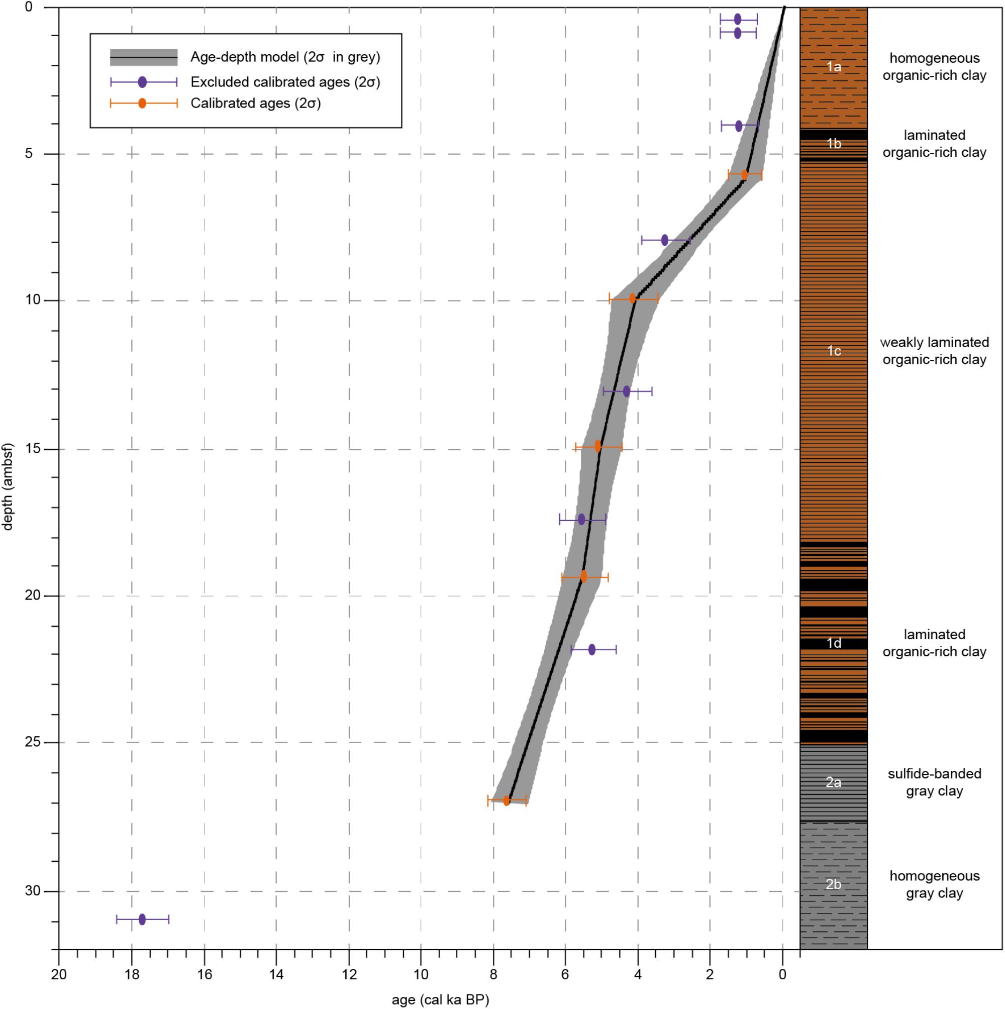
Figure 2. Calibrated sample ages, age-depth model and lithology for Integrated Ocean Drilling Program Expedition 347 Core M0063D. Calibrated ages (2σ) of samples that have been excluded from the age-depth model are indicated in purple. Calibrated ages (2σ) of samples that have been used for the age-depth model are indicated in orange. The black line represents the age-depth model, the gray area represents 2σ. Lithology and sedimentological units are obtained from Andrén et al. (2015).
Unit 2 is composed of gray clay. Subunit 2b (33.29–27.59 ambsf) consists of homogeneous gray clay. In Subunit 2a (27.59–25.06 ambsf) the dark gray clay is characterized by weak iron sulfide-stained laminations. Unit 1 consists of organic-rich clays, with homogeneous, weakly laminated and distinct laminated intervals. Prominent colorful laminated organic-rich clays characterize Subunit 1d (25.06–18.16 ambsf). Subunit 1c (18.16–5.23 ambsf) is composed of more homogeneous black organic-rich clays, though some weak laminations are visible. Subunit 1b (5.23–4.13 ambsf) shows laminations in the black clay. Subunit 1a (4.13–0 ambsf) is composed of black organic-rich clay, no sedimentary features are visible, probably because this section experienced a high degree of gas expansion.
Methods
Age-Depth Model
One sample of benthic foraminifera was dated but found to be coated with calcite which resulted in a too young age. Due to the lack of datable macrofossils, a total of 13 bulk sediment samples from core M0063D have been radiocarbon analyzed by Beta Analytic (Table 1). An age-depth model was presented by Obrochta et al. (2017) based on 7 of these dates. Using this age-depth model on our proxies gave less reliable results and we therefore decided to scrutinize the 13 dated levels to produce an alternative model. By studying the sediment core images, several dates were rejected as they were from sediments that might have been disturbed during the coring process. One date (Beta418038;1720 ± 30) from possibly disturbed sediment, however, is backed by a very similar one from core M0063C (Beta 418207; 1760 ± 30) at similar depth, 5.835 ambsf and 5.22 mcd, respectively, and was therefore included. The presented age-depth model for site M0063 (Figure 2) is based on 5 calibrated radiocarbon dates (14C dates published in Obrochta et al., 2017) from the upper ∼27 ambsf (Table 1). It is worth noting that the age-depth model assumes that the top of the core has an age of -63 year BP as the year of coring was 2013. Considering the coring method, however, it is not likely that the very soft and water saturated very topmost sediments were recovered (Andrén et al., 2015).
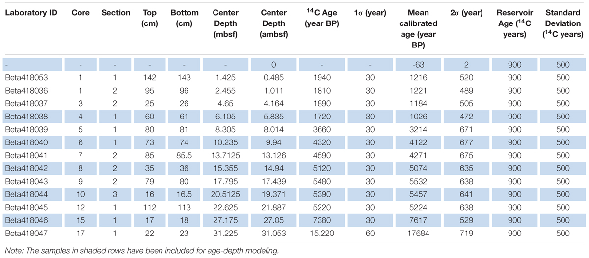
Table 1. Calibrated radiocarbon dates from Integrated Ocean Drilling Program Expedition 347 Site M0063, Hole D bulk sediment samples.
The age-depth modeling was performed using the age-modeling software CLAM version 2.2 (Blaauw, 2010). Linear interpolation was carried out between dated levels with 10000 iterations using a specially generated calibration dataset based on the IntCal 13 calibration curve (Reimer et al., 2013). A reservoir age (R) and a standard deviation of 900 and 500 14C years, respectively, were used in this age-depth model. These constraints have been used to make our alternative age-depth model comparable to the one presented by Obrochta et al. (2017) and are based on the regional bulk sediment R variability given by Lougheed et al. (2017). All subsequent ages discussed refer to calibrated ages in years before AD 1950 (cal ka BP). The mean sedimentation rate in the upper c. 27 ambsf is 3.5 mm/yr with the highest rate, 8.7 mm/y, recorded between c. 14.9 and 19.3 ambsf.
Siliceous Microfossils
A total of 54 sediment samples from the upper 30 ambsf (c. 50 cm resolution) were freeze-dried, after which a known weight of sediment was subsampled for the preparation of samples for diatom analysis. Diatom suspensions were prepared according to standard procedures (Battarbee, 1986), and microspheres were added to allow for diatom concentration reconstructions following Battarbee and Kneen (1982). Samples were analyzed for siliceous microfossils using an Olympus BX 51 light microscope with Nomarski differential interference contrast at 1000x magnification and oil immersion. Counting procedures were carried out according to Schrader and Gersonde (1978). When possible, at least 300 diatom valves (excluding Chaetoceros spp. resting spores) were counted and identified to species level in each sample. If diatom abundance was too low to reach 300 valves in one slide, a total of at least 1000 microspheres was counted. Diatom valves were identified to species level according to Cleve-Euler (1951; 1952; 1953a, b, 1955); Krammer and Lange-Bertalot (1975; 1988; 1991a, b); Snoeijs (1993); Snoeijs and Vilbaste (1994); Snoeijs and Kasperovičienė (1996); Snoeijs and Potapova (1995); Snoeijs and Balashova (1998); Witkowski et al. (2000).
Chaetoceros spp. resting spores were counted as well, but not identified to species level, except for Chaetoceros mitra epivalves. Since the hypovalves of C. mitra were not distinguished from other Chaetoceros spp. resting spores, only the presence of C. mitra is used. The group Chaetoceros spp. resting spores will from now on be addressed as resting spores and include Chaetoceros mitra. Silicoflagellates and ebridians were counted and identified to species level.
The relative abundance (%) of the diatom taxa was calculated including resting spores in the total diatom sum. For the diatom stratigraphy the diatom species that have a relative abundance of at least 4% in one level were plotted, after confirming that no important indicator species were left out due to this cut. Life-forms (benthic or pelagic) and salinity preferences (Supplementary Table S1) of the diatom taxa were obtained from the intercalibration guides of Snoeijs (1993); Snoeijs and Vilbaste (1994); Snoeijs and Potapova (1995); Snoeijs and Kasperovičienė (1996); Snoeijs and Balashova (1998). The diatom species present, were grouped into four different salinity affinity groups, i.e., freshwater (F), brackish-freshwater (BF), and brackish-marine (BM), and a group unknown (U). Group U contains both species with unknown affinity, and diatoms that could not be identified to species level. Relative abundances of the salinity affinity groups were calculated. The ratio of benthic to pelagic diatom taxa (B/P ratio) was calculated using relative abundances. Absolute abundances of siliceous microfossils were calculated according to Battarbee and Kneen (1982) and expressed in numbers of valves per gram dry weight (gdw).
Terrestrial and Marine Palynomorphs
For the analysis of terrestrial and marine palynomorph assemblages, 35 samples of c. 1 cm thickness were subsampled from 0 to c. 25 ambsf (c. 100 cm resolution). Pilot studies (Andrén et al., 2015) indicated that material between c. 25 and 30 ambsf (Unit 2) was barren of well-preserved palynomorphs. Per sample, 1 to 6 g of sediment was processed using standard palynological techniques for marine sediments (HCl and HF treatment and sieving with 7-μm mesh; Kotthoff et al., 2008). Lycopodium marker spores were added to the samples to calculate palynomorph concentrations (Stockmarr, 1971). Approximately 200 pollen grains were identified and counted per sample under 400 to 1000x magnification. Differentiation of triporate grains of Carpinus and Corylus, was based on general shape (triangular-flattened versus spheroidal), while size could only be used to some degree (compare section “Pollen”). Organic-walled dinocysts and Radiosperma were also determined and counted. The concentration of Radiosperma is given in specimens per gram dry weight of sediment (gdw). Since the amount of dinocysts varied greatly over the analyzed material, with several samples being almost barren, we could not aim at counting a fixed sum of dinocysts per samples. Therefore, good preservation of dinocysts under hypoxic conditions may result in artificial peaks in laminated sediments. To avoid this artifact we present dinocysts percentages in relation to the pollen sum [in accordance with Kotthoff et al. (2017)]. The general development of dinocysts concentrations is described in the results section. We have measured the process length of encountered O. centrocarpum cysts. The average spine length encountered is 3.96 μm, which is in accordance with findings by Willumsen et al. (2013). However, since the number of specimens measured is low we do not present a process-length plot in the results section.
Benthic Foraminifera
A total of 191 samples of 2-cm core length (20 ml sediment) were prepared for foraminiferal analyses (c. 20 cm resolution). The samples were weighted wet and washed through sieves with mesh sizes of 63, 100, and 1000 μm. The sample fractions were subsequently dried at 40°C and weighed. The 100–1000 μm fraction was used for the foraminiferal assemblage analysis; all foraminifera present in this fraction were counted. Benthic foraminifera were identified to species level to exclude reworked Quaternary and pre-Quaternary specimens from calculations of the abundance of allochthonous benthic foraminifera. These benthic foraminiferal concentrations were calculated as number of specimens per gram wet weight of sediment (gww).
Geochemistry
For geochemistry, a total of 203 samples from the upper 30 ambsf were analyzed for carbon and biogenic silica content (c. 20 cm resolution). Total carbon (TC) was measured on dry samples using a Euro EA from Hekatech; and an EA 1110 CHN from CE-Instruments (GC-based methods). Since sediments from the open Baltic Sea contain almost no carbonate carbon (Andrén et al., 2015; Hardisty et al., 2016; Warden et al., 2017; Häusler et al., 2018), trends in TC were regarded as trends in organic carbon. Biogenic silica (BSi) was determined after basic extraction: 50 mg of dry sample matter was treated with 100 ml 1 M NaOH for 40 min at 80°C in shaking steel backers. The resulting suspensions were then centrifuged, filtrated, and prepared for Si-analysis with ICP-OES. The method was developed and modified as proposed by Müller and Schneider (1993), and quality assurance was tested by including standard material from Conley (1998).
Results
Age-Depth Model
The homogeneous clay in Unit 2b was not suitable for radiocarbon dating (Table 1), due to the low content of organic carbon in the sediments (Figure 5; Olsson, 1979). Therefore, no reliable ages could be obtained for Subunit 2b and for the lower limit of Subunit 2a. According to the age-depth model (Figure 2), sediments in lithological Subunit 1d were deposited between 7.1 and 5.4 cal ka BP, Subunit 1c between 5.4 and 0.9 cal ka BP, Subunit 1b between 0.9 and 0.7 cal ka BP, and Subunit 1a between 0.7 cal ka BP and present-day.
Siliceous Microfossils
The samples analyzed in Subunit 2b are all barren of siliceous microfossils (Figures 3–5), this is likely a combined effect of poor diatom preservation and low diatom production, since the carbon content is low as well. In Subunit 2a diatom preservation is considered moderate to good. This subunit is characterized by a shift from a complete freshwater diatom assemblage to an assemblage with more brackish-marine diatom species (Figure 4). No silicoflagellates (Figure 4) nor ebridians are present (Figure 5). At 27.6 ambsf the freshwater pelagic taxa Aulacoseira islandica and Stephanodiscus neoastraea dominate the assemblage (Figure 3). A completely barren sample is found at 27.2 ambsf (Figure 3). At 26.4 ambsf (7.4 cal ka BP) the diatom concentration increases (Figure 5) and the assemblage is still characterized by freshwater species, this time dominated by Cyclotella radiosa and Pantocsekiella comensis (Figure 3). At c. 25.6 ambsf (7.2 cal ka BP), the diatom concentration is too low to reach 300 counts (Figure 3). The brackish-freshwater epiphyte Amphora pediculus is recorded for the first time in the stratigraphy (Figure 3). Brackish-marine Chaetoceros spp. resting spores also have their first occurrence here, albeit in low abundances (Figure 5).
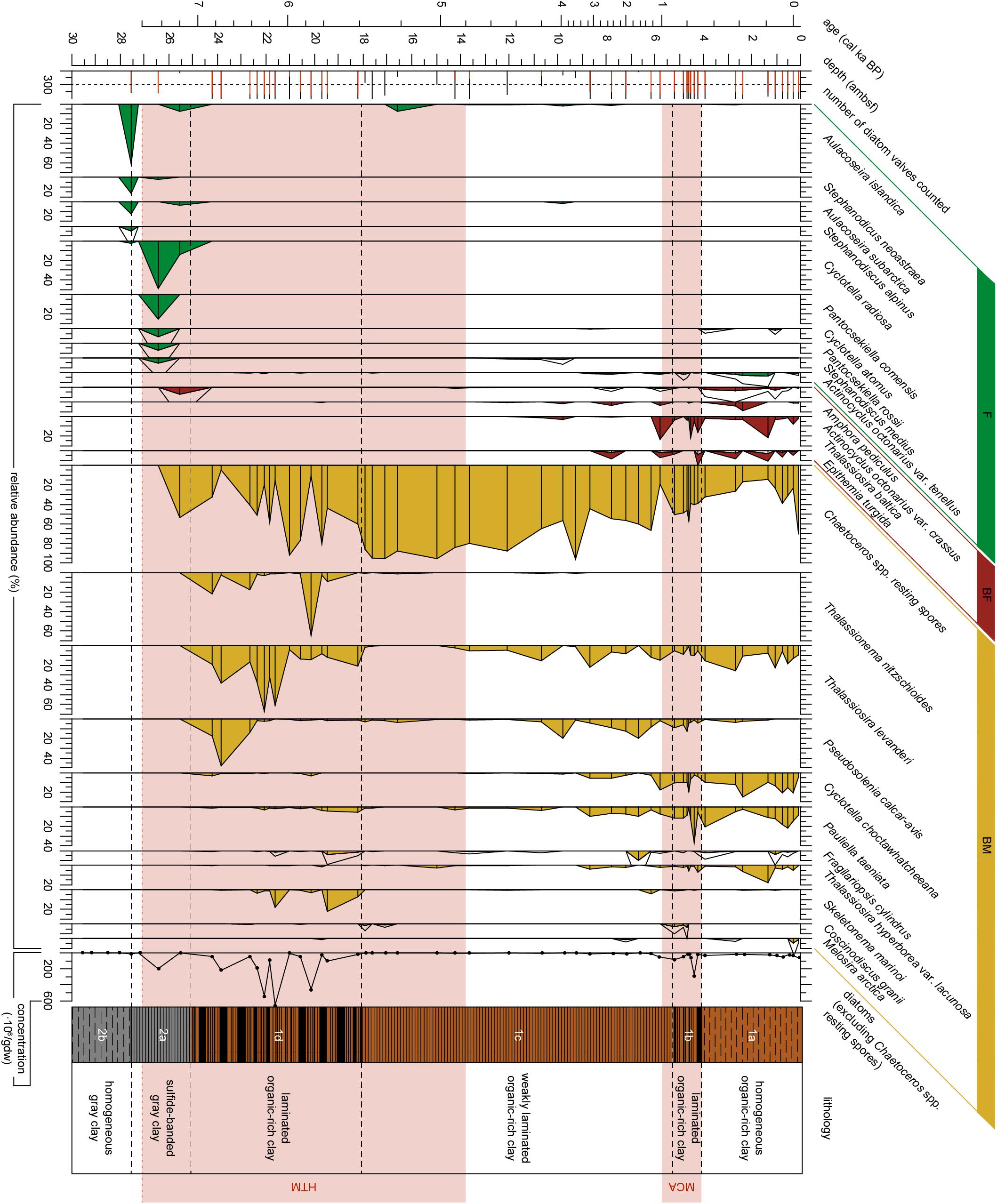
Figure 3. Diatom stratigraphy for the upper ∼27 ambsf (adjusted meters below seafloor) of Integrated Ocean Drilling Program Expedition 347 core M0063D. The number of diatoms counted are indicated in red for diatom valves other than Chaetoceros spp. resting spores, the black bars indicate the number of Chaetoceros spp. resting spores counted, the dotted vertical line represents a count of 300. Relative abundances (%) of diatom taxa with an abundance of 4% or greater in any sample versus depth (ambsf) are plotted as filled areas, for diatom species with a relative abundance <10% a 4x exaggeration is added by the black line. Analyzed levels are indicated by black bars. Diatoms are arranged by their environmental preference with respect to salinity (F, Freshwater affinity; BF, Brackish-Freshwater affinity; BM, Brackish-Marine affinity), and by their first occurrence. Absolute abundance of vegetative diatom valves in millions of valves per gram dry weight (gdw). The warm climate anomalies Holocene Thermal Maximum (HTM, 8–4.8 cal ka BP, Seppä et al., 2009) and Medieval Climate Anomaly [MCA, 1.0 - 0.7 cal ka BP(MCA, 1.0 – 0.7 cal ka BP, Mann et al., 2009)] are represented by the light red areas. Lithology and sedimentological units are obtained from Andrén et al. (2015).
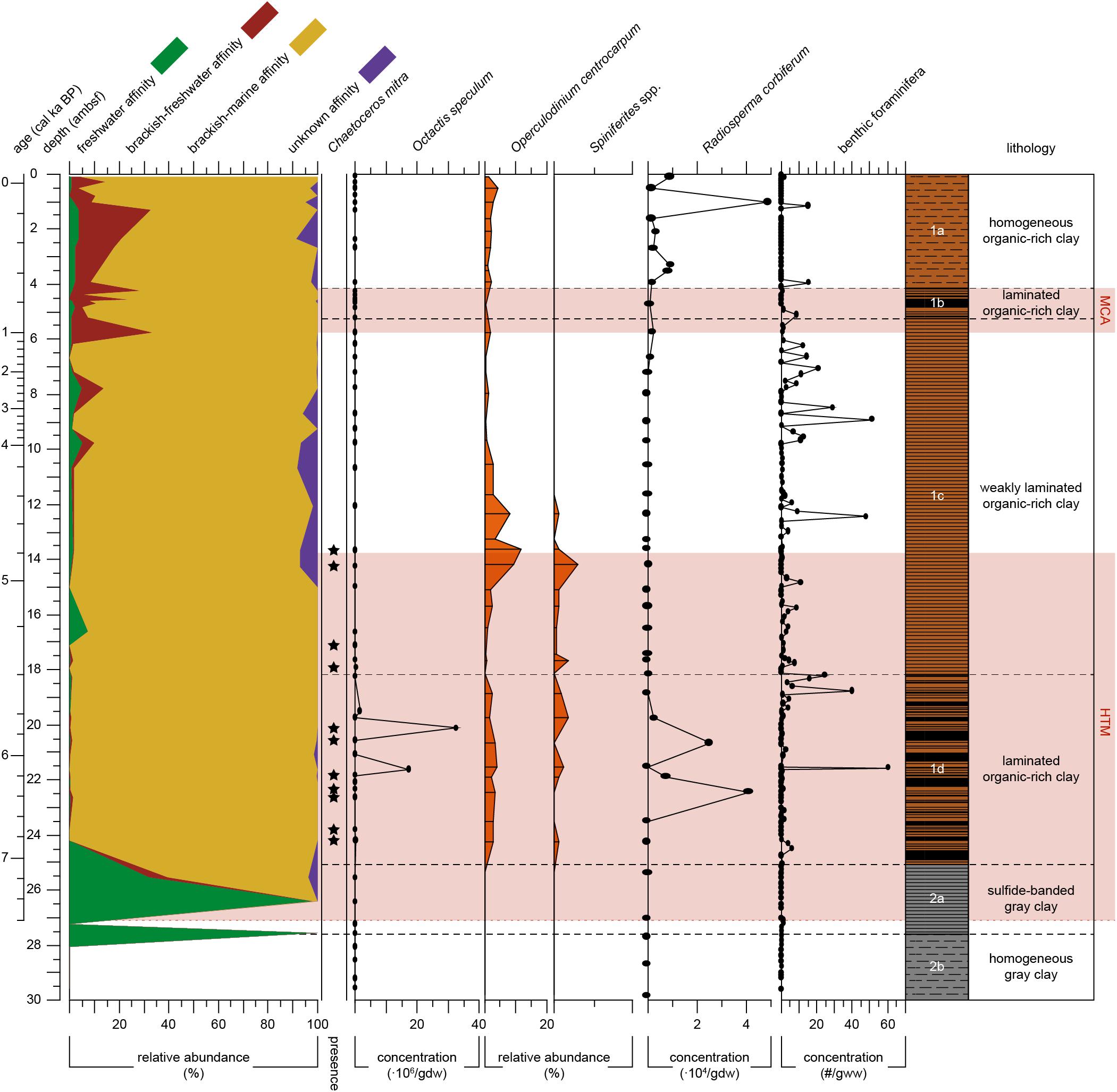
Figure 4. Proxy records for salinity of Integrated Ocean Drilling Program Expedition 347 core M0063D plotted versus depth (adjusted meters below seafloor). Relative abundance of diatom salinity-based affinity groups (i.e., freshwater. brackish-freshwater. brackish-marine and unknown) are plotted as different color-filled areas. Presence of Chaetoceros mitra resting spores are indicated by black dots. Absolute abundance of the silicoflagellate Octatis speculum [× 106 skeletons/gram dry weight (gdw)]. Relative abundances (% related to pollen sum) of dinoflagellate cysts Operculodinium centrocarpum and Spiniferites spp. Absolute abundances of Radiosperma corbiferum (× 104/gdw). Absolute abundance of benthic foraminifera in number per gram wet weight (gww). The warm climate anomalies Holocene Thermal Maximum (HTM, 8–4.8 cal ka BP, Seppä et al., 2009) and Medieval Climate Anomaly [MCA, 1.0 – 0.7 cal ka BP(MCA, 1.0 – 0.7 cal ka BP, Mann et al., 2009)] are represented by the light red areas. Lithology and sedimentological units are obtained from Andrén et al. (2015).
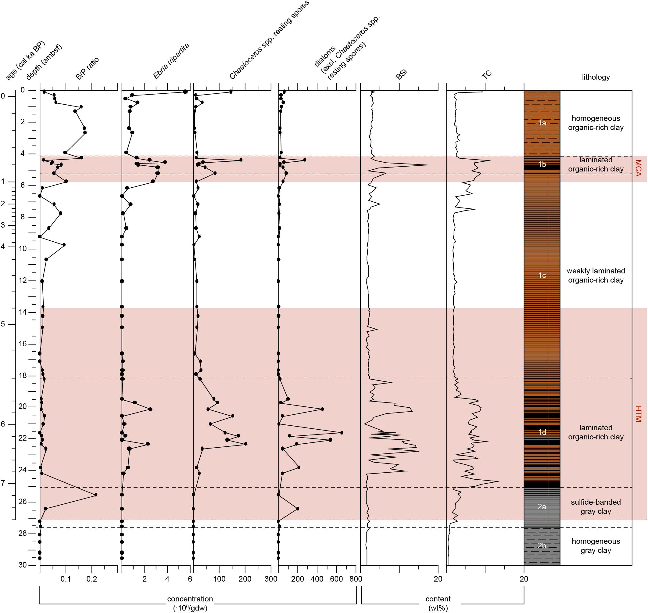
Figure 5. Proxy records for primary productivity of Integrated Ocean Drilling Program Expedition 347 core M0063D plotted versus depth (adjusted meters below seafloor). The ratio of benthic to pelagic diatoms (B/P ratio) has no unit. Absolute abundance of Ebria tripartita, Chaetoceros spp. resting spores and vegetative diatom valves in millions of valves per gram dry weight (gdw). Biogenic silica (BSi) and total carbon (TC) content of the sediments (wt%). The warm climate anomalies Holocene Thermal Maximum (HTM, 8–4.8 cal ka BP, Seppä et al., 2009) and Medieval Climate Anomaly [MCA, 1.0 – 0.7 cal ka BP(MCA, 1.0 - 0.7 cal ka BP, Mann et al., 2009)] are represented by the light red areas. Lithology and sedimentological units are obtained from Andrén et al. (2015).
Subunit 1d (7.1–5.4 cal ka BP) is dominated by brackish-marine diatom taxa (Figure 4), with no freshwater species present (Figure 3). Diatom preservation is good in this subunit. The brackish-marine pelagic taxa Pseudosolenia calcar-avis, Thalassiosira levanderi, Skeletonema marinoi, and Thalassionema nitzschioides all have their highest relative abundances in this zone (Figure 3). The marine pelagic silicoflagellate Octactis speculum only occurs here, and Chaetoceros mitra resting spores mainly occur in this subunit (Figure 4). The ebridian Ebria tripartita occurs in relatively high numbers at 22.3 (6.3 cal ka BP) and 20.1 (5.7 cal ka BP) ambsf (Figure 5). Concentrations of both resting spores and other diatom valves are highest in this Subunit (Figure 5).
Subunit 1c (5.4–0.9 cal ka BP) is still dominated by brackish-marine diatom species (Figure 4). However, the concentration of diatom valves other than Chaetoceros spp. resting spores between 18 and 9 ambsf (5.4–3.4 cal ka BP) is too low to reach 300 counts. Chaetoceros spp. resting spores dominate the diatom assemblage (Figure 3), though its concentration is relatively low compared to Subunit 1d (Figure 5). In this part of Subunit 1c the more heavily silicified diatom species might be over-represented, due to dissolution of the more finely silicified diatom species. Between 8.7 and 5.2 ambsf (3.1–0.9 cal ka BP), the number of brackish-freshwater taxa increases (Figure 4.), diatom preservation is moderate, with relatively high fragmentation of valves. Thalassionema nitzschioides is no longer present, whereas Thalassiosira levanderi and Pseudosolenia calcar-avis are still abundant, albeit with a lower relative abundance compared to Subunit 1d (Figure 3). Increased abundances of Cyclotella choctawhatcheeana, Pauliella taeniata, Fragilariopsis cylindrus, Thalassiosira baltica and Thalassiosira hyperborea var. lacunosa are recorded (Figure 3). The B/P ratio, concentrations of Ebria tripartita, and both resting spores and other diatom valves show an increasing trend towards the top of this subunit (Figure 5).
Subunit 1b (0.9–0.7 cal ka BP) is characterized by a relatively high abundance of the brackish-freshwater taxon Thalassiosira baltica and sea-ice associated taxon Pauliella taeniata (Figure 3). The brackish-marine pelagic taxa Thalassiosira levanderi, Pseudosolenia calcar-avis, and Cyclotella choctawhatcheeana are all relatively abundant in this Subunit (Figure 3). The concentration of Ebria tripartita is relatively high, as well as the concentrations of both resting spores and other diatoms (Figure 5). Preservation of diatom valves is good in this subunit.
Subunit 1a (0.7 cal ka BP-present) is characterized by increasing abundances of fresh- and brackish-freshwater diatom species (Figure 3). The relative abundances of the pelagic freshwater taxon Actinocyclus octonarius var. tenellus, brackish-freshwater taxon A. octonarius var. crassus, brackish-freshwater epiphytes Epithemia turgida and Amphora pediculus increase (Figure 3). Thalassiosira baltica decreases, though increasing again at 1.3 ambsf (0.2 cal ka BP). Thalassiosira levanderi, Pauliella taeniata, and Cyclotella choctawhatcheeana contribute considerably to the assemblage. Thalassiosira hyperborea var. lacunosa increases towards the top whereas Pseudosolenia calcar-avis decreases (Figure 3). The B/P ratio is highest in this subunit, Ebria tripartita is present in intermediate numbers, both resting spore and vegetative diatom abundance are relatively low (Figure 5). At 1.0 ambsf (0.3 cal ka BP), the relative abundance of freshwater and brackish-freshwater taxa decreases (Figure 4). The brackish-marine species Pseudosolenia calcar-avis and Thalassionema nitzschioides are not present. The benthic to planktic ratio decreases towards the core top, whereas concentrations of both Ebria tripartita and resting spores show an increase in the uppermost sample, the diatom concentration increases as well, albeit not as much (Figure 5). Preservation of diatom valves is considered moderate to good in this subunit.
Pollen
Samples are almost barren of pollen in Unit 2 but appear, except for Picea, all at the same level at 25.4 ambsf (7.1 cal ka BP) in Subunit 2b (Figure 6). Pollen preservation was good in nearly all samples, but grains appeared smaller than in recent samples in several cases. In Unit 1, pollen grains are frequent and well preserved. The pollen spectra for Subunit 1d (7.1–5.4 cal ka BP) shows a general dominance of Pinus (pine) pollen grains, but lower percentages than the following subunits. Picea (spruce) is almost absent in this unit. Pollen of warmth loving broad-leaved trees such as Alnus (alder), Quercus (oak), Ulmus (elm), Carpinus and Corylus (hornbeam and hazel, combined in Coryloideae), and Tilia (linden), show relatively high percentages in Subunit 1d compared to the units above. Poaceae pollen percentages vary around 1.3 % in this unit. The transition to Subunit 1c (5.4 cal ka BP) is marked by an increase in bisaccate pollen (Pinus and Picea), with Pinus percentages >50% and a general decrease in several broad-leaved-tree pollen, particularly Alnus and Corylus, and, slightly later, Tilia (Figure 6). Corylus and Ulmus show generally lower percentages in Subunit 1c compared to the lower subunit, while Picea is consistently present, with a slight increasing trend. One sample at 12.3 ambsf (4.5 cal ka BP) reveals particularly high Pinus values, paired with decreases in pollen of several broad-leaved taxa. Subunit 1b (0.9–0.7 cal ka BP) is only reflected in one sample of the palynological record (Figure 6). It is characterized by particularly low Pinus occurrences and a relative increase in Picea, Betula, and Alnus. Subunit 1a (0.7 cal ka BP-present) shows an increase in Betula and Alnus at 2.7 ambsf (0.4 cal ka BP). A decrease in Betula and Alnus follows and is coeval with an increase of bisaccate pollen. In the uppermost sample Betula increased again and is coeval with a decrease in Pinus (Figure 6). Pollen of herb taxa and Poaceae (grasses) are generally rare (usually < 2%) in this record, which is in accordance with other Holocene records from the central Western Baltic (e.g., Påhlsson and Bergh Alm, 1985; Thulin et al., 1992). Only in the uppermost samples (<2 ambsf, 0.3 cal ka BP), Poacea pollen show average percentages >2%, coevally with a decrease in pollen of broad-leaved trees.
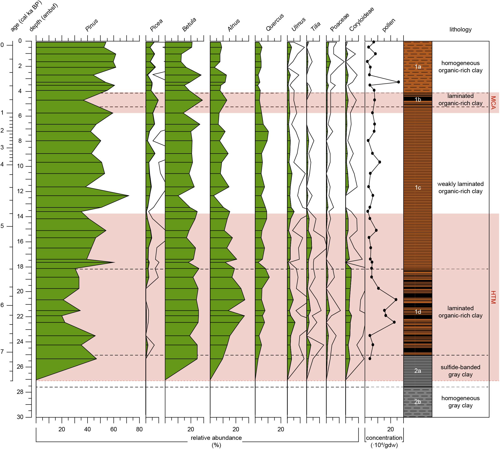
Figure 6. Pollen record of Integrated Ocean Drilling Program Expedition 347 core M0063D plotted versus depth (adjusted meters below seafloor). Relative abundance of selected pollen taxa (%) indicated by green-filled areas, abundances of pollen taxa that have a relative abundance <10% are in addition 4x exaggerated (black line). Carpinus and Corylus (hornbeam and hazel) are combined in the group Coryloideae. Analyzed levels are indicated by the black lines. Pollen concentrations in x 104/gram dry weight. The warm climate anomalies Holocene Thermal Maximum (HTM, 8–4.8 cal ka BP, Seppä et al., 2009) and Medieval Climate Anomaly [MCA, 1.0 – 0.7 cal ka BP(MCA, 1.0 – 0.7 cal ka BP, Mann et al., 2009)] are represented by the light red areas. Lithology and sedimentological units are obtained from Andrén et al. (2015).
Marine Palynomorphs
Dinocyst concentration is generally low in the analyzed samples (on average < 2000 cysts/gdw compared to ∼65000 pollen grains/gdw). A record from the Fårö Deep (Figure 1) shows significantly higher concentrations (Willumsen et al., 2013). In our record two cyst types of gonyaulacoid dinoflagellates have been found in certain intervals in higher occurrences. These belong to the taxa Operculodinium centrocarpum and Spiniferites spp. Lingulodinium cysts, which are known from the southwestern Baltic Sea (Kotthoff et al., 2017), were not encountered. This is in accordance with results of Ning et al. (2016), who found Lingulodinium cysts in only very low concentrations in a coastal sediment core from the Western Gotland Basin. The concentration of Radiosperma in certain units is higher compared to the record from Fårö Deep (Willumsen et al., 2013).
Dinocysts and Radiosperma are not present in Unit 2. In Subunit 1d (7.1–5.4 cal ka BP), both Spiniferites spp. and O. centrocarpum are present (Figure 4), but the abundances of Spiniferites spp. cysts compared to pollen grains are low (<2%). Radiosperma concentration shows two peaks, which are coeval with particularly low Spiniferites spp. values. In the lower part of Subunit 1c (c. 5.4–4.4 cal ka BP), the relative abundance of dinocysts compared to pollen increases to the highest values within the record (>10% at 13.6 ambsf; 4.8 cal ka BP; Figure 4). The absolute abundance of dinocysts is slightly lower compared to Subunit 1d. In the upper part (4.4–0.9 cal ka BP) of Subunit 1c Spiniferites spp. is not present, and both relative (Figure 4) and absolute abundances of O. centrocarpum are low. Remains of Radiosperma are almost absent in Subunit 1c, though its concentration increases slightly in the uppermost part (from 2.0 cal ka BP).
Subunit 1b (0.9–0.7 cal ka BP) reveals no particular difference to the subunits underneath. Subunit 1a shows a higher concentration of Radiosperma within the samples, with two peaks at 3.3 (0.6 cal ka BP) and 1.0 ambsf (0.1 cal ka BP, Figure 4). Spiniferites spp. remains absent in Subunits 1b and 1a, while O. centrocarpum shows increasing relative values compared to pollen grains within Subunit 1a (0.7 cal ka BP-present).
Benthic Foraminifera
Total foraminiferal abundances are overall low throughout core M0063 (Figure 4). Only calcareous benthic foraminifera are present in the samples. Foraminifera are only found in relatively high concentrations in certain intervals, and many samples are found to be barren. The specimens are generally not well-preserved, which indicates some effect of carbonate dissolution. Three different allochthonous species have been identified, the dominant species is Elphidium clavatum, with Elphidium albiumbilication and Elphidium incertum also present in lower numbers in intervals where foraminifera are most abundant. In addition, the samples also contain some reworked glacial Quaternary (e.g., Cassidulina reniforme) and pre-Quaternary (mainly upper Cretaceous) species that have not been included in the analyses.
Foraminifera are present in low but very gradually increasing numbers in Subunit 2b (Figure 4). In subunit 2a a first, minor peak in concentration occurs at c. 27.2 ambsf. In Unit 1, low foraminiferal abundances are regularly interrupted by foraminiferal abundance peaks. Clusters of such peaks in benthic foraminiferal concentrations are common from the top (7.1 cal ka BP) of Subunit 1d until the end of Subunit 1b (0.7 cal ka BP) with maximum occurrences between 19–18 ambsf (Subunit 1d/1c, 5.5–5.4 cal ka BP), at 12.8 ambsf (Subunit 1c, 4.6 cal ka BP), and 9.8–5 ambsf (Subunit 1c/1b, 3.9–0.9 cal ka BP).
Geochemistry
Biogenic Silica (BSi)
In Unit 2 the biogenic silica content is relatively low, varying between 1.3 and 3.0 wt% (Figure 5). In Subunit 1d, at 24.0 ambsf (6.8 cal ka BP) a sudden increase is recorded, i.e., from 1.4 to 11.5 wt%. In Subunit 1d (7.1–5.4 cal ka BP), biogenic silica content is on average relatively high (6.0 wt%), shifting between maxima of 15.0 wt%, and minima as low as 1.0 wt%. In the lower part (5.4–2.3 cal ka BP) of Subunit 1c, values are relatively stable, on average 2.0 wt%. An increasing trend is recorded in the upper part of Subunit 1c, starting at 7.5 ambsf (2.3 cal ka BP). In Subunit 1b, the highest biogenic silica content is recorded (17.3 wt%, 0.8 cal ka BP). In Subunit 1a values are again relatively stable, on average 2.9 wt%.
Total Carbon (TC)
In Subunit 2b, the carbon content is low, on average 0.7 wt% (Figure 5). In Subunit 2a, values increase to an average of 2.8 wt%. In Subunit 1d (7.1–5.4 cal ka BP) a sudden increase in carbon from 1.8 to 13.2 wt% is recorded, the latter is the maximum value in this record. In this subunit values are high, on average 6.7 wt%, though they are shifting between minima of 1.9 wt% and maxima of 13.2 wt%. At 19.4 ambsf (0.6 cal ka BP) a sharp decrease is recorded from 7.4 to 2.3 wt%. In the lower part (5.4–2.4 cal ka BP) of Subunit 1c, values are relatively stable, on average 2 wt%. In the upper part of Subunit 1c, values gradually increase, starting at 7.7 ambsf (2.4 cal ka BP). In Subunit 1b, values continue to gradually increase to a peak of 10.9 wt% (0.8 cal ka BP). After this peak, values decrease once again and are relatively stable in Subunit 1a, with an average of 2.6 wt%. In the uppermost sediments, carbon content increases to values as high as 9.3 wt%.
Discussion
Accuracy of the Age-Depth Model
The lithology, age-depth model, and diatom stratigraphy of M0063D confirm that the studied sediments were deposited during the Holocene, more specifically the Ancylus Lake and Littorina Sea stages (e.g., Lepland et al., 1999; Westman and Sohlenius, 1999; Andrén et al., 2000b) as well as more recent years. However, considering uncertainties introduced by both bulk reservoir ages and core expansion due to escaping gas, the accuracy of our age-depth model needs to be addressed. Therefore, we compare our organic matter record to that of two records in the vicinity of site M0063 (Supplementary Figure S2). Radiocarbon dating for core 9303 (250 m water depth; Figure 1; Bianchi et al., 2000) was carried out using bulk sediments, whereas for core M86-1a/36 (437 m water depth; Figure 1; Häusler et al., 2017) benthic foraminifera were used. This comparison reveals an age discrepancy at the termination of the high primary productivity period commonly attributed to the HTM. Our age-depth model suggests that this period ends at 5.4 cal ka BP, whereas organic matter content in the other records remains relatively high until c. 4 cal ka BP. Since it is highly unlikely that organic matter production has been this dissimilar between neighboring sites, we consider our age-depth model to be inaccurate in this part of the record. Four bulk sediment samples between 14.5 and 21.9 ambsf all have ages between c. 5.1 and 5.5 14C ka BP (Table 1), this indicates that bulk sediment ages in this section are less reliable. Pollen data from Lakes Holtjärnen and Klotjärnen in eastern Sweden (Giesecke, 2005) imply consistent occurrences of Picea around 5.2 cal ka BP, while records from the south coast of Sweden (compare e.g., Yu et al., 2005) show even later consistent occurrences. In western Estonia, Latvia and Lithuania Picea was well established at c. 6 cal ka BP (Giesecke and Bennett, 2004) and the pollen could very well have been transported to site M0063 both with wind and water currents. In our marine pollen record, Picea occurrences without interruptions start at ∼5.8 cal ka BP (Figure 6). Even if the appearance of Picea cannot be used as a precise marker, these findings support our assumption that for the interval of the HTM, our age model implies too old ages. Accordingly, we conclude that the exact timing of the termination of this high primary productivity period in our record is not provided by our age-depth model. Nevertheless, this inaccuracy does not hinder discussing mechanisms responsible for observed changes in our proxy records.
Environmental Conditions in the Landsort Deep During the Middle and Late Holocene
Subunit 2b
The low carbon and biogenic silica content of the sediments and the low diatom abundance (Figure 5) indicate low primary productivity during deposition of Subunit 2b (Table 2). The homogeneous gray clays of Subunit 2b suggest a well-mixed and oxygenated water column (Table 2). However, very low abundances of benthic foraminifera (Figure 4) suggest minor marine influence in the bottom waters of Landsort Deep. Due to the absence of siliceous microfossils interpretations regarding surface water salinity cannot be made (Figures 3, 4).
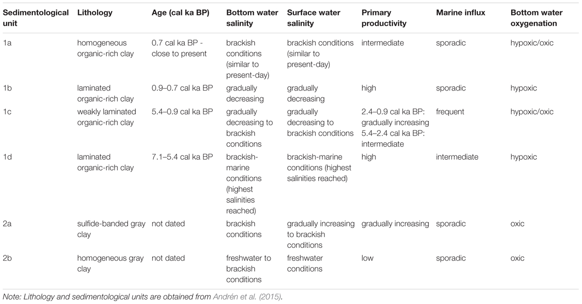
Table 2. Summary of salinity, primary productivity and bottom water oxygenation interpretations for Integrated Ocean Drilling Program Expedition 347 site M0063.
Low organic content and a well-oxygenated water body have been found characteristic for the Ancylus Lake stage (Sohlenius et al., 1996, 2001), a freshwater stage lasting from c. 10.7 to 9.8 ka BP (Andrén et al., 2011). Based on our proxy records, we suggest that the sediments in Subunit 2b cover part of the Ancylus Lake stage. A water body filled with discharged clay particles from the melting ice sheet led to a reduced extent of the photic zone (Winterhalter, 1992). Deglaciated land areas were exposed to wave action, which resulted in erosion of pristine soils into the water body. It is unlikely that the sediments in Subunit 2b are barren of siliceous microfossils only due to low primary production, since several studies show varying abundances of diatoms in the open Baltic Sea during the Ancylus Lake stage (Lepland et al., 1999; Westman and Sohlenius, 1999; Andrén et al., 2000a,b). Therefore, we presume diatom valves have been poorly preserved in this subunit due to dissolution.
Subunit 2a
The carbon content shows an increase around 7.6 cal ka BP, and gradually increases throughout Subunit 2a (Figure 5), indicating increased gross primary productivity (Table 2), hence nutrient availability. The large clear-water lake diatom species present in the oldest sediments of Subunit 2a (Figure 3), such as Aulacoseira islandica and Stephanodiscus neoastraea, demonstrate freshwater conditions in the surface waters. A minor peak in benthic foraminifera concentration at c. 7.6 cal ka BP Subunit 2a (Figure 4) signals a first minor influx of saline water to the deeper waters, while surface waters were still fresh (Table 2). After this first occurrence, benthic foraminifera become absent until c. 7.1 cal ka BP. The absence of marine palynomorphs (Figure 4) show surface water salinities are relatively low until c. 7.1 cal ka BP (Table 2). However, the diatom assemblage (Figure 3) implies considerable changes in surface water conditions and nutrient conditions from 7.4 to 7.1 cal ka BP.
In our record, the planktic species Cyclotella radiosa and Pantocsekiella comensis dominate the diatom assemblage at 7.4 cal ka BP (Figure 3). A similar assemblage is recorded between c. 8.2–7.9 cal ka BP in a sediment core from the Archipelago Sea (Tuovinen et al., 2008) and has been related to increased surface water salinity. Winder et al. (2009) have found that intensified stratification of the water column selects for the Cyclotella genus. The genus Cyclotella is also known to be a good competitor for nitrogen (Winder and Hunter, 2008), hence a nitrogen limited primary production may have allowed the fast-growing C. radiosa and P. comensis to dominate the diatom community. The shift from an oligotrophic freshwater diatom assemblage to an assemblage dominated by Cyclotella species coincides with a peak in diatom concentration (Figure 5). We suggest that both increased surface water salinity and nutrient availability played a role in this shift in species composition. Although the sample at 7.2 cal ka BP was almost barren of diatoms, the presence and Chaetoceros spp. resting spores (Figure 3) is indicative of a gradually increasing surface water salinity (Table 2).
The very low diatom abundance, increase in diatom diversity, and an assemblage dominated by periphytic fresh- and brackish-freshwater diatom species have been found characteristic for the Initial Littorina Sea stage in the open Baltic Sea (Westman and Sohlenius, 1999; Andrén et al., 2000a,b; Sohlenius et al., 2001). This stage is the time-transgressive transitional phase between the Ancylus Lake stage and Littorina Sea stage (Andrén, 1999; Andrén et al., 2000a,b), often referred to as the Mastogloia Sea in the coastal zone (Miettinen, 2004). Andrén et al. (2000a) identified the Initial Littorina Sea stage in a diatom record from the Eastern Gotland Basin and dated it to last from c. 8.3–7 cal ka BP. During this stage brackish conditions developed gradually throughout the basin, due to the interplay between sea level rise and subsidence of sills in the Danish Straits (Sohlenius et al., 2001). The sediments almost barren of diatoms deposited during this transitional stage have been suggested to be related to the effects of resuspension of sediments due to marine water inflow (Westman and Sohlenius, 1999). The occurrence of benthic species is likely due to increased transport form littoral zones, due to a changing surface circulation caused by the transgression of the Baltic Sea.
Subunit 1d (c. 7.1–5.4 cal ka BP)
The laminated sediments of Subunit 1d (Figure 2) imply hypoxic conditions prevailed during the time of deposition (Table 2). Carbon content shows a sharp increase at 7.1 cal ka BP, and remains relatively high until c. 5.6 cal ka BP (Figure 5). It has been argued that organic carbon is better preserved during anoxic bottom conditions, and therefore higher organic carbon values do not necessarily indicate increased primary productivity (Sohlenius et al., 2001). However, our data also show a sharp increase in biogenic silica and diatom concentration at 6.8 cal ka BP (Figure 5), which points to increased diatom productivity (Table 2). In addition, the concentrations of both Ebria tripartita and Chaetoceros spp. resting spores increase at 6.4 cal ka BP. Ebridians are cosmopolitan, marine, heterotrophic flagellates that have a rather widespread distribution (Korhola and Grönlund, 1999). It is suggested that ebridians are indicative for increased nutrient levels (Witkowski and Pempkowiak, 1995). The formation of Chaetoceros spp. resting spores are considered as indicators of previous high primary productivity events that resulted in nitrogen depletion in high salinity environments (Oku and Kamatani, 1997). Vegetative cells of the genus Chaetoceros are very lightly silicified, and therefore rarely found in the sediment record, in contrast their resting spores are heavily silicified and usually well preserved.
The species composition of the brackish-marine diatom assemblage (Figure 3) implies the highest surface water salinities indicated in our samples (Table 2). Pseudosolenia calcar-avis is a common marine species in tropical and subtropical waters (Viličić et al., 2009), and does not occur in the present Baltic Sea (Snoeijs and Kasperovičienė, 1996). Thalassionema nitzschioides is a widely distributed marine neritic species (Hasle and Syvertsen, 1997), favored by both warm and saline water conditions. At present it is not occurring in basins north of the Bornholm Basin (Snoeijs and Vilbaste, 1994). Chaetoceros mitra (Figure 4) is common in the present North Sea, but not found in the Baltic Sea nowadays, due to its low salinity (Snoeijs and Kasperovičienė, 1996; Hasle and Syvertsen, 1997). Resting spores of this species are only present in the older part of the Littorina Sea stage (Andrén et al., 2000a,b; Witak et al., 2011). Octactis speculum is an exclusively marine pelagic silicoflagellate requiring high salinity (Chang et al., 2017). In this core it is only present between c. 6.8 and 5.4 cal ka BP (Figure 4). Similar siliceous microfossil assemblages were found in other studies from the Baltic Proper (Thulin et al., 1992; Westman and Sohlenius, 1999; Andrén et al., 2000a), and are suggested to reflect maximum marine conditions during the Littorina Sea stage. Relatively saline surface water conditions are also indicated in our record by the first appearance of marine palynomorphs at c. 7.1 cal ka BP (Figure 4). Radiosperma is generally more abundant in our record compared to that of the Fårö Deep (Willumsen et al., 2013), where an increase in concentration was recorded at c. 8 cal ka BP. Ning et al. (2017) find an increase in Radiosperma at c. 7 cal ka BP in the Blekinge coast. In our record an increase is recorded at c. 6.5 cal ka BP (Figure 4). These differences in timing suggest that water depth and/or distance to the coast is an important factor in the distribution of this taxon.
Benthic foraminiferal concentrations fluctuate in this subunit. A minor peak at c. 6.9 cal ka BP (Figure 4)indicates the onset of relatively consistently reoccurring events of influx of saline water from the North Sea (Table 2). The still relatively low concentrations of benthic foraminifera after this peak are likely a result of a stratified water column with unfavorable oxygen conditions for benthic foraminifera. Periods with low bottom-water oxygenation would cause decrease or disappearance of benthic foraminifera, while periods of higher bottom-water oxygen concentration would allow the re-establishment of a benthic foraminiferal fauna. The high carbon content and lithology of the sediment also points towards low bottom-water oxygenation. It may have resulted in dissolution of foraminiferal tests accentuating the low number of calcareous benthic foraminifera in the deposits. The varying foraminiferal concentrations throughout this period point to fluctuating influence from the North Sea (Table 2).
Subunit 1c (c. 5.4–0.9 cal ka BP)
Carbon and biogenic silica content, and diatom concentrations are relatively low between 5.4 and 2.4 cal ka BP (Figure 5). The presence of Chaetoceros spp. resting spores, albeit in low numbers, suggests a slightly higher primary productivity compared to the Initial Littorina Sea stage. Although interpretations are not accurate due to small diatom concentrations, some implications for changing surface water salinity are provided by the diatom record. Chaetoceros spp. resting spores, Chaetoceros mitra resting spores, and the proboscis of Pseudosolenia calcar-avis are relatively heavily silicified and are thus expected to be preserved in the sediments. Whereas Chaetoceros spp. resting spores are abundant in most of this sequence, Pseudosolenia calcar-avis is only found in low numbers, and Chaetoceros mitra resting spores do not appear after c. 4.7 cal ka BP. This suggests a decrease in surface water salinities (Table 2), which is supported by the absence of the heavily silicified silicoflagellate Octactis speculum (Figure 4). The absence of Radiosperma may also point to lower salinity (Figure 4). Ning et al. (2017) find a similar decrease slightly earlier (c. 6.5 cal ka BP) at the Blekinge coast of Sweden. The absolute abundance of dinocysts within this interval is lower than in the sediments below, but this may be a preservation signal. The increase in relative abundance of dinocysts (Figure 4) indicates that the salinity of the surface waters is still high enough for both Spiniferites spp. and O. centrocarpum until c. 4.4 cal ka BP. These relatively high values of Spiniferites compared to the rest of the record are again in accordance with findings by Ning et al. (2017). After c. 4.4 cal ka BP, less saline surface water conditions probably lead to the decrease in Operculodinium and absence of Spiniferites cysts.
At c. 4.4 cal ka BP the diatom assemblage has an increased abundance of brackish-freshwater diatom taxa, and benthic diatom taxa are present (Figure 3). It is unlikely that benthic diatoms were abundant in the autochthonous living diatom assemblage in Landsort Deep because the photic zone cannot have reached such depths. The increased benthic to pelagic diatom ratio (Figure 5) therefore most likely indicates a change in the circulation pattern, bringing in benthic diatoms from the littoral zone, due to transgression and/or increased discharge from land. Concurrently, the appearance of more brackish-freshwater diatom taxa suggests a decreased salinity in the surface waters. Pseudosolenia calcar-avis occurs in this sequence, whereas other taxa which were abundant during the most marine phase have disappeared (e.g., Thalassionema nitzschioides, Chaetoceros mitra resting spores, Octactis speculum). Among the marine palynomorphs, Spiniferites cysts also vanished, and both Operculodinium cysts and Radiosperma decreased in abundance. This infers a drop in surface water salinities, although surface waters were still more saline than seen in the area today, since P. calcar-avis is still present. In contrast, the benthic foraminifera show a more consistent, albeit still fluctuating, presence in the sediments between c. 5.4 and 0.9 cal ka BP. This may, to some extent, be due to reduced post-mortem dissolution, but may also be linked to increased bottom-water ventilation either from increased subsurface inflow of marine waters or increased wind speeds.
Carbon and biogenic silica content show an increasing trend starting at c. 2.4 cal ka BP and coincide with increasing concentrations of Ebria tripartita. Diatom concentrations do not demonstrate any pronounced increases in this time-span, which may be a bias of the relatively high fragmentation of the diatom frustules in this sequence. Cyclotella choctawhatcheeana becomes one of the major contributors in the diatom assemblage from here on. This is a diatom taxon which has been referred to as a warm-water species (Hällfors, 2004), though also associated with anthropogenic disturbances and increasing eutrophication in the Baltic Sea (Andrén et al., 2000a; Weckström and Juggins, 2006). Based on these findings, we suggest that primary productivity increased during this period (Table 2).
Subunit 1b (c. 0.9–0.7 cal ka BP)
The highest carbon content is recorded in this subunit, at c. 0.8 cal ka BP (Figure 5) and coincides with a peak in diatom abundance. Biogenic silica also has a distinct peak, though slightly earlier. The discrepancy between these peaks remains unclear from this study. These peaks and the increased concentrations of Ebria tripartita and Chaetoceros spp. resting spores suggest increased primary productivity during this period (Table 2).
The diatom record shows no clear signs of increased surface water salinity compared to Subunit 1c (Figure 3). Diatom species Thalassiosira baltica, Pauliella taeniata, and Thalassiosira hyperborea var. lacunosa have been associated with sea ice (Snoeijs and Weckström, 2010). The increased abundance of these species and the accompanying decrease of Pseudosolenia calcar-avis illustrate decreased surface water salinities and a more extensive ice-coverage during winters. Relatively low abundances of Operculodinium cysts and Radiosperma (Figure 4) do not point to increased surface water salinities either. Benthic foraminiferal concentrations are relatively low, though a peak at c. 0.9 cal ka BP (Figure 4) indicates bottom water oxygenation (Table 2).
Subunit 1a (c. 0.7 cal ka BP-Present)
Carbon and biogenic silica content show a decreasing trend, though still slightly higher compared to before Subunit 1b (Figure 5). Resting spore and Ebria tripartita concentrations show a similar decreasing trend, ebridians are present in higher numbers compared to before Subnit 1b. This decreased but slightly higher primary productivity (Table 2) might be a combined influence of both a cooler climate and increased anthropogenic influence. The pollen record (Figure 6) corroborates an anthropogenic influence; even though cereal taxa have not been distinguished from other Poaceae in the framework of this project, we suggest that the consistent occurrence of Poaceae pollen with values around 2% in the upper two ambsf, combined with decreased percentages of broad-leaved trees such as Quercus, may point to increased land use. Such an increase is also consistent with findings by Påhlsson and Bergh Alm (1985).
Between c. 0.9 and 0.2 cal ka BP, brackish-freshwater diatom species increase in abundance (Figure 4). The small centric diatom taxa Cyclotella choctawhatcheeana and Thalassiosira levanderi have a relatively high abundance, and the freshwater taxon Cyclotella atomus appears, though in low relative abundances (Figure 3). Ice-associated species Thalassiosira baltica and Thalassiosira hyperborea var. lacunosa also increase throughout this sequence. This suggests a further decrease in surface water salinity and more extensive ice-coverage during winter (Table 2). The minor relative increase of Operculodinium cysts remains unclear in this context but could be tied to changes in water temperature. The increase in Radiosperma cannot be interpreted unequivocally since its biology is not completely understood (compare e.g., Brenner, 2001; and Ning et al., 2017). It may be that this taxon took profit from the change to brackish-fresh conditions for a short interval while the conditions during subunit 1c were probably too marine. In the most recent sequence in this record (c. 0.2 cal ka BP-present), Pseudosolenia calcar-avis is not present any longer, most likely surface salinity reached present-day levels. Benthic foraminiferal concentrations are low throughout Subunit 1a (Figure 4), indicating reduced bottom water ventilation (Table 2).
During the last c. 150 years of the sediment record, pelagic diatoms show an increased abundance compared to the older part of Subunit 1a (Figure 5). Such a change in B/P ratio has been found in other studies as well (Andrén, 1999; Andrén et al., 2000a,b), and is interpreted as a result of increased nutrient availability. Increased nutrient load leads to turbid waters and a shallower photic zone, unfavorable for benthic species. Increasing abundance of Ebria tripartita, Chaetoceros resting spores and increased carbon content (Figure 5) do support increased nutrient availability, hence increased primary productivity (Table 2).
Implications for the Development of Hypoxic Conditions in the Landsort Deep
The laminated Subunits 1d and 1b illustrate that the two main periods of hypoxia found throughout the Baltic Proper (Zillén et al., 2008) are recorded in our sediment core from the Landsort Deep. Here we discuss the relative importance of observed changes in salinity and primary productivity in relation to these two periods of hypoxia. A summary of our findings is presented in Table 2.
Hypoxia During the Holocene Thermal Maximum
Our proxy records show that bottom waters were the first to become more saline, followed by gradually increasing primary productivity and eventually surface waters becoming more saline before the onset of laminated sediments in Subunit 1d (Table 2). This succession can be explained by the establishment of a warmer climate commonly attributed to the HTM. In our pollen record (Figure 6), Subunit 1d is characterized by a higher pollen concentration compared to subsequent intervals. Broad-leaved tree pollen such as Alnus, Ulmus, Tilia, and Corylus all have relatively high relative abundances (compare to Seppä et al., 2015). Seppä et al. (2009) reconstructed warmer and/or more humid conditions until c. 5.8 ka BP compared to the conditions afterwards.
Increasing sill depths in the Baltic basin enhanced the inflow of saline and oxygenated water from the North Sea. Frequent inflows to the Baltic basin led to gradually increasing primary productivity by enhancing the availability of phosphorous. Marine water itself is enriched in phosphorous (Bianchi et al., 2000) but it also reduces binding of phosphorous in sediments (Caraco et al., 1990). Excess availability of phosphorous results in a nitrogen limited primary production. This, and higher surface water temperatures, favor nitrogen fixing cyanobacteria blooms (Bianchi and McCave, 1999; Kabel et al., 2012). The increase in carbon in our record is not accompanied by an increase in biogenic silica. Therefore, primary production might have been dominated by cyanobacteria rather than diatoms. The idea of a phosphorous-enriched water column is supported by the abundance of Cyclotella spp. around 7.4 cal ka BP. Reconstructed sea surface temperatures in a parallel core (M0063C) show that the threshold temperature for cyanobacteria was reached in Subunit 2a (Papadomanolaki et al., 2018). In the same parallel core high molybdenum concentrations are recorded in Subunit 2a and 1d (Hardisty et al., 2016), which have been suggested to be indicative for the presence of cyanobacteria blooms (Kunzendorf et al., 2001).
A halocline developed due to the inflow of highly saline North Sea water into the deep waters of the Baltic Sea basin. As soon as the water column became stratified and bottom waters became hypoxic several feedback mechanisms amplified the release of phosphorous from sediments (Emeis et al., 2000; Slomp, 2013). The sudden increase and peak in carbon content at the onset of the laminated sequence was likely due to a sudden release of phosphorus from the sediments during the transition from oxic to anoxic bottom water conditions (Emeis et al., 2000). Phosphorous continued to be released due to the establishment of hypoxic conditions and amplified primary productivity. The decomposition of organic material produced in turn sustains hypoxic conditions in the bottom waters.
The return to only weakly laminated sediments in Subunit 1c are related to the termination of this extensive hypoxic period. Similar sequences have been found in other records of the Baltic Basin (Westman and Sohlenius, 1999; Andrén et al., 2000a; Zillén et al., 2008), dated to c. 4–2 ka BP. Westman and Sohlenius (1999) suggest this homogeneous section was a result of a quick regression at the Öresund, which led to a decrease in inflowing marine waters, which in turn led to decreased nutrient upwelling, hence decreased primary productivity, allowing bottom waters to become oxic again and recolonization of burrowing animals. Furthermore, humid climate conditions (Zillén et al., 2008) likely led to more freshwater input from the drainage area resulting in decreased surface water salinity.
Our pollen record shows a relative increase in the taphonomically more robust bisaccate pollen grains (particularly Pinus) which probably points to less warm/humid conditions in summer for the time interval reflected in Subunit 1. We cannot completely rule out, though, that this relative increase of taphonomically more robust bisaccate grains may to some degree be caused by the end of dysoxic conditions in the sediments. Our proxy record suggests gradually decreasing surface water salinities in Subunit 1c, but the very low abundances of siliceous microfossils do not allow for reliable interpretations. The still relatively high abundance of marine palynomorphs demonstrate that surface water salinities did not drop to very low values. This is supported by the findings of Papadomanolaki et al. (2018), who found no considerable changes in surface water salinity. The fluctuating abundance of benthic foraminifera indicate fluctuating salinity and/or oxygen conditions at the sea floor. In contrast, primary productivity decreased considerably. Therefore, it is likely that it was not decreased salinity that was responsible for the termination of this hypoxic period (Subunit 1d) but rather decreased temperatures.
Hypoxia During the Medieval Climate Anomaly
The second period of prominent laminated sediments (Subunit 1b) is commonly attributed to changing climate conditions during the MCA. Benthic foraminiferal concentrations confirm reduced bottom-water oxygenation. The MCA is reflected in the pollen record as increased percentages of warmth-loving taxa like Alnus at the cost of taxa like Pinus (Figure 6). As for the previous hypoxic period, a gradual development in our proxy records is apparent and starts in the top of Subunit 1c.
The increasing B/P ratio and the highly fragmented diatom frustules in the upper sediments of Subunit 1c suggest increased influence from the littoral zone. As discussed before, the increasing abundance of C. choctwhatcheeana could point to eutrophication. Therefore, the increasing primary productivity during this period may be related to more nutrient input from land. This increased nutrient input could be due to increased freshwater discharge from the drainage area as a result of humid climate conditions, and/or human-induced eutrophication. Increased freshwater discharge would lead to both freshening of surface waters and a changed water circulation. Zillén and Conley (2010) suggest that anthropogenic forcing through increased nutrient input from the drainage area might have influenced the primary productivity in the Baltic Sea during these times. Recent studies from the Finnish and Swedish coast find no evidence of anthropogenic forcing during the MCA (Jokinen et al., 2018; Ning et al., 2018).
The diatom stratigraphy suggests that hypoxic conditions in Subunit 1b have not been due to pronounced salinity changes, but rather due to increased primary productivity. In addition to the above discussed possible increased nutrient load from land the warmer climate itself has likely played a major role in this increased productivity. The warmer conditions during this period led to increased production of organic carbon resulting in more oxygen consumption during degradation. The increased oxygen consumption in the deeper waters stratified the water column which further promoted hypoxia at the bottom waters and increased primary production in the surface waters due to the release of phosphorus. Cyanobacteria might once again have had a major contribution to the organic carbon pool during this time, due to the phosphorous-enrichment and warmer sea surface temperatures (Kabel et al., 2012). In M0063C high molybdenum concentrations were recorded in this subunit (Hardisty et al., 2016), and thus support the idea of cyanobacteria blooms during this time. The increase in absolute abundance of Chaetoceros resting spores could be pointing to a nitrogen depleted sea.
Primary productivity significantly decreased after this period of hypoxia, and the homogeneous sediments of Subunit 1a suggest increased bottom-water ventilation. Benthic foraminiferal concentrations are, however relatively low. The diatom assemblage reflects gradually decreasing surface water salinities getting close to the present-day values. The termination of this hypoxic period is likely due to the cooling of the climate after the MCA.
Conclusion
Based on microfossil, carbon, and silica data we reconstructed the variability in surface and bottom water salinity and primary productivity in the Landsort Deep over the past c. 7600 years. We assessed the relative importance of such changes for the establishment and termination of hypoxic conditions at the sea floor and conclude the following:
1. increased bottom water salinity set the stage for the development of hypoxic conditions during the Holocene Thermal Maximum
2. the return to oxic conditions after this first period of hypoxia is mainly due to decreased surface water temperatures
3. no considerable changes in salinity are recorded before, during and, after the hypoxic period attributed to the Medieval Climate Anomaly
Our results emphasize the impact of natural climate forcing on the development of hypoxic conditions in the Baltic Sea. Although human-induced eutrophication is likely the most important forcing factor of the current spreading of hypoxia, future changes in salinity and productivity induced by both naturally and anthropogenically forced climate dynamics, can be of similar importance. Hence, a good understanding of such climatic processes is of importance when designing action plans to improve the status of the Baltic Sea ecosystem.
Author Contributions
TA, EA, and FvW contributed to the conception and design of the study. FvW performed the siliceous microfossil analysis. UK and DW performed the palynomorph analysis. A-SF performed the foraminiferal analysis. MM performed the geochemistry analysis. TA provided the age-depth model. FvW harmonized all data, provided figures, and wrote the first draft of the manuscript. TA, UK, DW, M-SS, and MM wrote sections of the manuscript. All authors contributed to manuscript revision, read and approved the submitted version.
Funding
This research was supported by the Foundation for Baltic and East European Studies (Grants 1562/3.1.1/2013 and 2207/3.1.1/2014), the Swedish Research Council (Grant 826-2012-5114), the Carlsberg Foundation (IVAR-347 project) and Geocenter Denmark (DAN-IODP-SEIS project), the Independent Research Fund Denmark (Grant 7014-00113B, G-Ice), and the German Research Foundation (DFG, projects Ko3944/6-1 and Ko3944/8–1).
Conflict of Interest Statement
The authors declare that the research was conducted in the absence of any commercial or financial relationships that could be construed as a potential conflict of interest.
Acknowledgments
This study used samples from IODP Expedition 347, and we are very grateful to IODP and ESSAC for funding and organizing the expedition. We thank the crew and science party of IODP Exp. 347, as well as the technical staff at MARUM, Bremen, for their support during the expeditions off- and onshore phases. We are also grateful for technical support from the different laboratories involved in the study. Karen Luise Knudsen is thanked for discussion on foraminiferal species taxonomy and ecology. We also thank the reviewers and editor for giving constructive input which has helped to improve the manuscript.
Supplementary Material
The Supplementary Material for this article can be found online at: https://www.frontiersin.org/articles/10.3389/fmars.2019.00051/full#supplementary-material
References
Åkesson, C., Nielsen, A. B., Broström, A., Persson, T., Gaillard, M. J., and Berglund, B. E. (2015). From landscape description to quantification: a new generation of reconstructions provides new perspectives on Holocene regional landscapes of SE Sweden. Holocene 25, 178–193. doi: 10.1177/0959683614556552
Andersen, J. H., Carstensen, J., Conley, D. J., Dromph, K., Fleming-Lehtinen, V., Gustafsson, B. G., et al. (2017). Long-term temporal and spatial trends in eutrophication status of the Baltic Sea: eutrophication in the Baltic Sea. Biol. Rev. 92, 135–149. doi: 10.1111/brv.12221
Andrén, E. (1999). Holocene Environmental Changes Recorded by Diatom Stratigraphy in the Southern Baltic Sea. Stockholm: Stockholm University.
Andrén, E., Andrén, T., and Kunzendorf, H. (2000a). Holocene history of the Baltic Sea as a background for assessing records of human impact in the sediments of the Gotland Basin. Holocene 10, 687–702. doi: 10.1191/09596830094944
Andrén, E., Andrén, T., and Sohlenius, G. (2000b). The holocene history of the southwestern Baltic Sea as reflected in a sediment core from the Bornholm Basin. Boreas 29, 233–250. doi: 10.1111/j.1502-3885.2000.tb00981.x
Andrén, T., Björck, S., Andrén, E., Conley, D., Zillén, L., and Anjar, J. (2011). “The development of the Baltic Sea Basin during the last 130 ka,” in The Baltic Sea Basin, eds J. Harff, S. Björck, and P. Hoth (Berlin: Springer), 75–97.
Andrén, T., Jørgensen, B. B., Cotterill, C., Green, S., and the Iodp Expedition 347 Scientists. (2015). Proc. IODP. College Station TX: Integrated Ocean Drilling Program.
Battarbee, R. W. (1986). “Diatom analysis,” in Handbook of Holocene Palaeoecology and Palaeohydrology, ed. B. E. Berglund (Chichester: Wiley), 527–570.
Battarbee, R. W., and Kneen, M. J. (1982). The use of electronically counted microspheres in absolute diatom analysis. Limnol. Oceanogr. 27, 184–188. doi: 10.4319/lo.1982.27.1.0184
Bergstrom, S., and Carlsson, B. (1994). River runoff to the Baltic Sea: 1950-1990. AMBIO 23, 280–287.
Bianchi, G. G., and McCave, I. N. (1999). Holocene periodicity in North Atlantic climate and deep-ocean flow south of Iceland. Nature 397, 515–517. doi: 10.1038/17362
Bianchi, T. S., Engelhaupt, E., Westman, P., Andrén, T., Rolff, C., and Elmgren, R. (2000). Cyanobacterial blooms in the Baltic Sea: natural or human-induced? Limnol. Oceanogr. 45, 716–726. doi: 10.4319/lo.2000.45.3.0716
Björck, S. (1995). A review of the history of the Baltic Sea, 13.0-8.0 ka BP. Quat. Int. 27, 19–40. doi: 10.1016/1040-6182(94)00057-C
Blaauw, M. (2010). Methods and code for ‘classical’ age-modelling of radiocarbon sequences. Quat. Geochronol. 5, 512–518. doi: 10.1016/j.quageo.2010.01.002
Borzenkova, I., Zorita, E., Borisova, O., Kalniņa, L., Kisielienė, D., Koff, T., et al. (2015). “Climate change during the holocene (Past 12,000 Years),” in Proceedings of the Second Assessment of Climate Change for the Baltic Sea Basin Regional Climate Studies, (Cham: Springer), 25–49. doi: 10.1007/978-3-319-16006-1_2
Breitburg, D., Levin, L. A., Oschlies, A., Grégoire, M., Chavez, F. P., Conley, D. J., et al. (2018). Declining oxygen in the global ocean and coastal waters. Science 359:eaam7240. doi: 10.1126/science.aam7240
Brenner, W. (2001). Organic-walled microfossils from the central Baltic Sea, indicators of environmental change and base for ecostratigraphic correlation. Baltica 14, 40–51.
Caraco, N., Cole, J., and Likens, G. E. (1990). A comparison of phosphorus immobilization in sediments of freshwater and coastal marine systems. Biogeochemistry 9, 277–290. doi: 10.1007/BF00000602
Carstensen, J., Conley, D. J., Bonsdorff, E., Gustafsson, B. G., Hietanen, S., Janas, U., et al. (2014). Hypoxia in the Baltic Sea: biogeochemical cycles, benthic fauna, and management. AMBIO 43, 26–36. doi: 10.1007/s13280-013-0474-7
Chang, F. H., Sutherland, J., and Bradford-Grieve, J. (2017). Taxonomic revision of dictyochales (Dictyochophyceae) based on morphological, ultrastructural, biochemical and molecular data. Phycol. Res. 65, 235–247. doi: 10.1111/pre.12181
Cleve-Euler, A. (1951). Die Diatomeen von Schweden und Finnland. T. 1. Stockholm: Almqvist & Wiksell.
Cleve-Euler, A. (1952). Die Diatomeen von Schweden und Finnland. T. 5, Schluss. Stockholm: Almqvist & Wiksell.
Cleve-Euler, A. (1953a). Die Diatomeen von Schweden und Finnland. T. 2, Arraphideae, Brachyraphideae. Stockholm: Almqvist & Wiksell.
Cleve-Euler, A. (1953b). Die Diatomeen von Schweden und Finnland. T. 3, Monoraphideae, Biraphideae 1. Stockholm: Almqvist & Wiksell.
Cleve-Euler, A. (1955). Die Diatomeen von Schweden und Finnland. T. 4, Biraphideae 2. Stockholm: Almqvist & Wiksell.
Conley, D. J. (1998). An interlaboratory comparison for the measurement of biogenic silica in sediments. Mar. Chem. 63, 39–48. doi: 10.1016/S0304-4203(98)00049-8
Conley, D. J., Carstensen, J., Aigars, J., Axe, P., Bonsdorff, E., Eremina, T., et al. (2011). Hypoxia is increasing in the coastal zone of the Baltic Sea. Environ. Sci. Technol. 45, 6777–6783. doi: 10.1021/es201212r
Conley, D. J., Humborg, C., Rahm, L., Savchuk, O. P., and Wulff, F. (2002). Hypoxia in the Baltic Sea and basin-scale changes in phosphorus biogeochemistry. Environ. Sci. Technol. 36, 5315–5320. doi: 10.1021/es025763w
Diaz, R. J., and Rosenberg, R. (2008). Spreading dead zones and consequences for marine ecosystems. Science 321, 926–929. doi: 10.1126/science.1156401
Elken, J., and Matthäus, W. (2008). “Physical system description,” in Proceedings of the Assessment of Climate Change for the Baltic Sea Basin Regional Climate Studies, (Berlin: Springer), 379–389.
Emeis, K. C., Struck, U., Blanz, T., Kohly, A., and Voβ, M. (2003). Salinity changes in the central Baltic Sea (NW Europe) over the last 10000 years. Holocene 13, 411–421. doi: 10.1191/0959683603hl634rp
Emeis, K. C., Struck, U., Leipe, T., Pollehne, F., Kunzendorf, H., and Christiansen, C. (2000). Changes in the C, N, P burial rates in some Baltic Sea sediments over the last 150 years—relevance to P regeneration rates and the phosphorus cycle. Mar. Geol. 167, 43–59. doi: 10.1016/S0025-3227(00)00015-3
Flodén, T., and Brännström, B. (1965). En thumperprofil genom landsortsdjupet. Geol. Fören. Stockh. Förh. 87, 337–346. doi: 10.1080/11035896509448917
Funkey, C. P., Conley, D. J., Reuss, N. S., Humborg, C., Jilbert, T., and Slomp, C. P. (2014). Hypoxia sustains cyanobacteria blooms in the Baltic Sea. Environ. Sci. Technol. 48, 2598–2602. doi: 10.1021/es404395a
Giesecke, T. (2005). Holocene dynamics of the southern boreal forest in Sweden. Holocene 15, 858–872. doi: 10.1191/0959683605hl859ra
Giesecke, T., and Bennett, K. D. (2004). The holocene spread of Picea abies (L.) Karst. in Fennoscandia and adjacent areas. J. Biogeogr. 31, 1523–1548. doi: 10.1111/j.1365-2699.2004.01095.x
Granéli, E., Wallström, K., Larsson, U., Granéli, W., and Elmgren, R. (1990). Nutrient limitation of primary production in the Baltic Sea Area. AMBIO 19, 142–151.
Gustafsson, B. G., and Westman, P. (2002). On the causes for salinity variations in the Baltic Sea during the last 8500 years. Paleoceanography 17, 12.1–12.14. doi: 10.1029/2000PA000572
Hällfors, G. (2004). “Checklist of Baltic Sea phytoplankton species (including some heterotrophic protistan groups),” in Proceedings of the Baltic Sea Environmental, (Helsinki: HELCOM).
Hardisty, D. S., Riedinger, N., Planavsky, N. J., Asael, D., Andrén, T., Jørgensen, B. B., et al. (2016). A holocene history of dynamic water column redox conditions in the Landsort Deep, Baltic Sea. Am. J. Sci. 316, 713–745. doi: 10.2475/08.2016.01
Hasle, G. R., and Syvertsen, E. E. (1997). “Chapter 2 - marine diatoms,” in Identifying Marine Phytoplankton, ed. C. R. Tomas (San Diego, CA: Academic Press), 5–385.
Häusler, K., Dellwig, O., Schnetger, B., Feldens, P., Leipe, T., Moros, M., et al. (2018). Massive Mn carbonate formation in the Landsort Deep (Baltic Sea): hydrographic conditions, temporal succession, and Mn budget calculations. Mar. Geol. 395, 260–270. doi: 10.1016/j.margeo.2017.10.010
Häusler, K., Moros, M., Wacker, L., Hammerschmidt, L., Dellwig, O., Leipe, T., et al. (2017). Mid- to late Holocene environmental separation of the northern and central Baltic Sea basins in response to differential land uplift. Boreas 46, 111–128. doi: 10.1111/bor.12198
Helcom. (2017). First Version of the “State of the Baltic Sea” report - June 2017 - to be Updated in 2018. Available at: http://stateofthebalticsea.helcom.fi
Jilbert, T., and Slomp, C. P. (2013). Iron and manganese shuttles control the formation of authigenic phosphorus minerals in the euxinic basins of the Baltic Sea. Geochim. Cosmochim. Acta 107, 155–169. doi: 10.1016/j.gca.2013.01.005
Jilbert, T., Slomp, C. P., Gustafsson, B. G., and Boer, W. (2011). Beyond the Fe-P-redox connection: preferential regeneration of phosphorus from organic matter as a key control on Baltic Sea nutrient cycles. Biogeosciences 8, 1699–1720. doi: 10.5194/bg-8-1699-2011
Jokinen, S. A., Virtasalo, J. J., Jilbert, T., Kaiser, J., Dellwig, O., Arz, H. W., et al. (2018). A 1500-year multiproxy record of coastal hypoxia from the northern Baltic Sea indicates unprecedented deoxygenation over the 20<sup>th</sup> century. Biogeosciences 15, 3975–4001. doi: 10.5194/bg-2018-25
Jonsson, P., Carman, R., and Wulff, F. (1990). Laminated sediments in the baltic: a tool for evaluating nutrient mass balances. AMBIO 19, 152–158.
Kabel, K., Moros, M., Porsche, C., Neumann, T., Adolphi, F., Andersen, T. J., et al. (2012). Impact of climate change on the Baltic Sea ecosystem over the past 1,000 years. Nat. Clim. Change 2, 871–874. doi: 10.1038/nclimate1595
Kononen, K. (2001). Eutrophication, harmful algal blooms and species diversity in phytoplankton communities: examples from the Baltic Sea. AMBIO J. Hum. Environ. 30, 184–189. doi: 10.1579/0044-7447-30.4.184
Korhola, A., and Grönlund, T. (1999). Observations of Ebria tripartita (Schumann) lemmermann in baltic sediments. J. Paleolimnol. 21, 1–8. doi: 10.1023/A:1008019504122
Kotthoff, U., Groeneveld, J., Ash, J. L., Fanget, A. S., Krupinski, N. Q., Peyron, O., et al. (2017). Reconstructing Holocene temperature and salinity variations in the western Baltic Sea region: a multi-proxy comparison from the little belt (IODP expedition 347, Site M0059). Biogeosciences 14, 5607–5632. doi: 10.5194/bg-14-5607-2017
Kotthoff, U., Pross, J., Müller, U. C., Peyron, O., Schmiedl, G., Schulz, H., et al. (2008). Climate dynamics in the borderlands of the aegean sea during formation of sapropel S1 deduced from a marine pollen record. Quat. Sci. Rev. 27, 832–845. doi: 10.1016/j.quascirev.2007.12.001
Krammer, K., and Lange-Bertalot, H. (1975). Süsswasserflora von Mitteleuropa. Bd 2, Bacillariophyceae, T. 1, Naviculaceae. Stuttgart: Fischer.
Krammer, K., and Lange-Bertalot, H. (1988). Süsswasserflora von Mitteleuropa. Bd 2, Bacillariophyceae, T. 2, Bacillariaceae, Epithemiaceae,Surirellaceae. Stuttgart: Fischer.
Krammer, K., and Lange-Bertalot, H. (1991a). Süsswasserflora von Mitteleuropa. Bd 2, Bacillariophyceae, T. 3, Centrales, Fragilariaceae, Eunotiaceae. Stuttgart: Fischer.
Krammer, K., and Lange-Bertalot, H. (1991b). Süsswasserflora von Mitteleuropa. Bd 2, Bacillariophyceae, T. 4, Achnanthaceae: Kritische Ergänzungen zu Navicula (Lineolatae) und Gomphonema. Stuttgart: Fischer.
Kunzendorf, H., Voss, M., Brenner, W., Andrén, T., and Vallius, H. (2001). Molybdenum in sediments of the central Baltic Sea as an indicator for algal blooms. Baltica 14, 123–130.
Lagerås, P. (2007). The Ecology of Expansion and Abandonment: Medieval and Post-Medieval Agriculture and Settlement in a Landscape Perspective. Stockholm: Riksantikvarieämbetet.
Lepland, A., Heinsalu, A., and Stevens, R. L. (1999). The pre-Littorina diatom stratigraphy and sediment sulphidisation record from the west-central Baltic Sea: Implications of the water column salinity variations. GFF 121, 57–65. doi: 10.1080/11035899901211057
Lepland, A., and Stevens, R. L. (1998). Manganese authigenesis in the Landsort Deep, Baltic Sea. Mar. Geol. 151, 1–25. doi: 10.1016/S0025-3227(98)00046-2
Leppäranta, M., and Myrberg, K. (2009). Physical Oceanography of the Baltic Sea. Berlin: Springer-Verlag. doi: 10.1007/978-3-540-79703-6
Lignell, R., Seppälä, J., Kuuppo, P., Tamminen, T., Andersen, T., and Gismervik, I. (2003). Beyond bulk properties: responses of coastal summer plankton communities to nutrient enrichment in the northern Baltic Sea. Limnol. Oceanogr. 48, 189–209. doi: 10.4319/lo.2003.48.1.0189
Lougheed, B. C., Obrochta, S. P., Lenz, C., Mellström, A., Metcalfe, B., Muscheler, R., et al. (2017). Bulk sediment 14C dating in an estuarine environment: how accurate can it be: estuarine bulk sediment 14C dating. Paleoceanography 32, 123–131. doi: 10.1002/2016PA002960
Mann, M. E. (2007). Climate over the past two millennia. Annu. Rev. Earth Planet. Sci. 35, 111–136. doi: 10.1146/annurev.earth.35.031306.140042
Mann, M. E., Zhang, Z., Hughes, M. K., Bradley, R. S., Miller, S. K., Rutherford, S., et al. (2008). Proxy-based reconstructions of hemispheric and global surface temperature variations over the past two millennia. Proc. Natl. Acad. Sci. 105, 13252–13257. doi: 10.1073/pnas.0805721105
Mann, M. E., Zhang, Z., Rutherford, S., Bradley, R. S., Hughes, M. K., Shindell, D., et al. (2009). Global signatures and dynamical origins of the little ice age and medieval climate anomaly. Science 326, 1256–1260. doi: 10.1126/science.1177303
Matthäus, W. (2006). The History of Investigation of Salt Water Inflows into the Baltic Sea- from the Early Beginning to Recent Results. Warnemünde: Baltic Sea Research Institute Warnemünde.
Matthäus, W., Nehring, D., Feistel, R., Nausch, G., Mohrholz, V., and Lass, H. U. (2008). “The inflow of highly saline water into the Baltic Sea,” in State and Evolution of the Baltic Sea, 1952-2005: A Detailed 50-Year Survey of Meteorology and Climate, Physics, Chemistry, Biology, and Marine Environment, eds R. Feistel, G. Nausch, and N. Wasmund (Hoboken, NJ: John Wiley & Sons, Inc), 265–309. doi: 10.1002/9780470283134.ch10
Meier, H. E. M., Andersson, H. C., Eilola, K., Gustafsson, B. G., Kuznetsov, I., Müller-Karulis, B., et al. (2011a). Hypoxia in future climates: a model ensemble study for the Baltic Sea. Geophys. Res. Lett. 38:L24608. doi: 10.1029/2011GL049929
Meier, H. E. M., Eilola, K., and Almroth, E. (2011b). Climate-related changes in marine ecosystems simulated with a 3-dimensional coupled physical-biogeochemical model of the Baltic Sea. Clim. Res. 48, 31–55. doi: 10.3354/cr00968
Meier, H. E. M., Höglund, A., Eilola, K., and Almroth-Rosell, E. (2017). Impact of accelerated future global mean sea level rise on hypoxia in the Baltic Sea. Clim. Dyn. 49, 163–172. doi: 10.1007/s00382-016-3333-y
Meier, H. E. M., Hordoir, R., Andersson, H. C., Dieterich, C., Eilola, K., Gustafsson, B. G., et al. (2012). Modeling the combined impact of changing climate and changing nutrient loads on the Baltic Sea environment in an ensemble of transient simulations for 1961–2099. Clim. Dyn. 39, 2421–2441. doi: 10.1007/s00382-012-1339-7
Miettinen, A. (2004). Holocene sea-level changes and glacio-isostasy in the Gulf of Finland, Baltic Sea. Quat. Int. 120, 91–104. doi: 10.1016/j.quaint.2004.01.009
Mohrholz, V., Dutz, J., and Kraus, G. (2006). The impact of exceptionally warm summer inflow events on the environmental conditions in the Bornholm Basin. J. Mar. Syst. 60, 285–301. doi: 10.1016/j.jmarsys.2005.10.002
Mohrholz, V., Naumann, M., Nausch, G., Krüger, S., and Gräwe, U. (2015). Fresh oxygen for the Baltic Sea — an exceptional saline inflow after a decade of stagnation. J. Mar. Syst. 148, 152–166. doi: 10.1016/j.jmarsys.2015.03.005
Müller, P. J., and Schneider, R. (1993). An automated leaching method for the determination of opal in sediments and particulate matter. Deep Sea Res. Part Oceanogr. Res. Pap. 40, 425–444. doi: 10.1016/0967-0637(93)90140-X
Neumann, T., Radtke, H., and Seifert, T. (2017). On the importance of major baltic inflows for oxygenation of the central Baltic Sea. J. Geophys. Res. Oceans 122, 1090–1101. doi: 10.1002/2016JC012525
Ning, W., Andersson, P. S., Ghosh, A., Khan, M., and Filipsson, H. L. (2017). Quantitative salinity reconstructions of the Baltic Sea during the mid-Holocene. Boreas 46, 100–110. doi: 10.1111/bor.12156
Ning, W., Ghosh, A., Jilbert, T., Slomp, C. P., Khan, M., Nyberg, J., et al. (2016). Evolving coastal character of a Baltic Sea inlet during the Holocene shoreline regression: impact on coastal zone hypoxia. J. Paleolimnol. 55, 319–338. doi: 10.1007/s10933-016-9882-6
Ning, W., Nielsen, A. B., Ivarsson, L. N., Jilbert, T., Åkesson, C. M., Slomp, C. P., et al. (2018). Anthropogenic and climatic impacts on a coastal environment in the Baltic Sea over the last 1000 years. Anthropocene 21, 66–79. doi: 10.1016/j.ancene.2018.02.003
Obrochta, S. P., Andrén, T., Fazekas, S. Z., Lougheed, B. C., Snowball, I., Yokoyama, Y., et al. (2017). The undatables: quantifying uncertainty in a highly expanded late glacial-holocene sediment sequence recovered from the deepest Baltic Sea basin—IODP Site M0063. Geochem. Geophys. Geosyst. 18, 858–871. doi: 10.1002/2016GC006697
Oku, O., and Kamatani, A. (1997). Resting spore formation of the marine planktonic diatom Chaetoceros anastomosans induced by high salinity and nitrogen depletion. Mar. Biol. 127, 515–520. doi: 10.1007/s002270050040
Olsson, I. (1979). A warning against radiocarbon dating of samples containing little carbon. Boreas 8, 203–207. doi: 10.1111/j.1502-3885.1979.tb00801.x
Påhlsson, I., and Bergh Alm, K. (1985). Pollen-analytical studies of the cores 14103-3 and 14102-1 from the Western Baltic. Striae 23, 74–82.
Papadomanolaki, N. M., Dijkstra, N., van Helmond, N. A. G. M., Hagens, M., Bauersachs, T., Kotthoff, U., et al. (2018). Controls on the onset and termination of past hypoxia in the Baltic Sea. Palaeogeogr. Palaeoclimatol. Palaeoecol. 490, 347–354. doi: 10.1016/j.palaeo.2017.11.012
Reimer, P. J., Bard, E., Bayliss, A., Beck, J. W., Blackwell, P. G., Ramsey, C. B., et al. (2013). IntCal13 and Marine13 radiocarbon age calibration curves 0–50,000 years cal BP. Radiocarbon 55, 1869–1887. doi: 10.1016/j.dib.2018.10.040
Reissmann, J. H., Burchard, H., Feistel, R., Hagen, E., Lass, H. U., Mohrholz, V., et al. (2009). Vertical mixing in the Baltic Sea and consequences for eutrophication – a review. Prog. Oceanogr. 82, 47–80. doi: 10.1016/j.pocean.2007.10.004
Renssen, H., Seppä, H., Crosta, X., Goosse, H., and Roche, D. M. (2012). Global characterization of the holocene thermal maximum. Quat. Sci. Rev. 48, 7–19. doi: 10.1016/j.quascirev.2012.05.022
Rosentau, A., Bennike, O., Uścinowicz, S., and Miotk-Szpiganowicz, G. (2017). “The Baltic Sea basin,” in Submerged Landscapes of the European Continental Shelf, eds N. C. Flemming, J. Harff, D. Moura, A. Burgess, and G. N. Bailey (Hoboken, NJ: John Wiley & Sons Ltd).
Schimanke, S., Meier, H. E. M., Kjellström, E., Strandberg, G., and Hordoir, R. (2012). The climate in the Baltic Sea region during the last millennium simulated with a regional climate model. Clim. Past 8, 1419–1433. doi: 10.5194/cp-8-1419-2012
Schrader, H. J., and Gersonde, R. (1978). “Diatoms and silicoflagellates,” in Micropaleontological Counting Methods and Techniques: an Exercise on an Eight Metres Section of the Lower Pliocene of Capo Rossello, Sicily Utrecht Micropaleontological Bulletins, eds W. J. Zachariasse, W. R. Riedel, A. Sanfilippo, R. R. Schmidt, M. J. Brolsma, and H. J. Schrader (Utrecht: Schotanus and Jens).
Seppä, H., Bjune, A. E., Telford, R. J., Birks, H. J. B., and Veski, S. (2009). Last nine-thousand years of temperature variability in Northern Europe. Clim. Past Discuss. 5, 1521–1552. doi: 10.5194/cpd-5-1521-2009
Seppä, H., Schurgers, G., Miller, P. A., Bjune, A. E., Giesecke, T., Kühl, N., et al. (2015). Trees tracking a warmer climate: the holocene range shift of hazel (Corylus avellana) in northern Europe. Holocene 25, 53–63. doi: 10.1177/0959683614556377
Slomp, C. P. (2013). Reconstructing the history of euxinia in a coastal sea. Geology 41, 523–524. doi: 10.1130/focus0420131.1
Snoeijs, P. (1993). Intercalibration and Distribution of Diatom Species in the Baltic Sea, Vol. 1. Uppsala: Opulus press.
Snoeijs, P., and Balashova, N. (1998). Intercalibration and Distribution of Diatom Species in the Baltic Sea, Vol. 5. Uppsala: Opulus press.
Snoeijs, P., and Kasperovičienė, J. (1996). Intercalibration and Distribution of Diatom Species in the Baltic Sea, Vol. 4. Uppsala: Opulus press.
Snoeijs, P., and Potapova, M. (1995). Intercalibration and Distribution of Diatom Species in the Baltic Sea, Vol. 3. Uppsala: Opulus press.
Snoeijs, P., and Vilbaste, S. (1994). Intercalibration and Distribution of Diatom Species in the Baltic Sea, Vol. 2. Uppsala: Opulus press.
Snoeijs, P., and Weckström, K. (2010). “Diatoms and environmental change in large brackish-water ecosystems,” in The Diatoms: Applications for the Environmental and Earth Sciences, eds J. P. Smol and E. F. Stoermer (Cambridge: Cambridge University Press), 287–308. doi: 10.1017/CBO9780511763175.016
Snowball, I., Korhola, A., Briffa, K. R., and Koç, N. (2004). “Holocene climate dynamics in Fennoscandia and the North Atlantic,” in Past Climate Variability Through Europe and Africa Developments in Paleoenvironmental Research, eds R. W. Battarbee, F. Gasse, and C. E. Stickley (Dordrecht: Springer),465–494.
Sohlenius, G., Emeis, K. C., Andrén, E., Andrén, T., and Kohly, A. (2001). Development of anoxia during the Holocene fresh–brackish water transition in the Baltic Sea. Mar. Geol. 177, 221–242. doi: 10.1016/S0025-3227(01)00174-8
Sohlenius, G., Sternbeck, J., Andrén, E., and Westman, P. (1996). Holocene history of the Baltic Sea as recorded in a sediment core from the Gotland Deep. Mar. Geol. 134, 183–201. doi: 10.1016/0025-3227(96)00047-3
Stockmarr, J. (1971). Tablets with spores used in absolute pollen analysis. Pollen Spores 13, 615–621.
Storch von, H., Omstedt, A., Pawlak, J., and Reckermann, M. (2015). “Introduction and Summary,” in Proceedings of the Second Assessment of Climate Change for the Baltic Sea Basin Regional Climate Studies, (Cham: Springer), 1–22.
Tamminen, T., and Andersen, T. (2007). Seasonal phytoplankton nutrient limitation patterns as revealed by bioassays over Baltic Sea gradients of salinity and eutrophication. Mar. Ecol. Prog. Ser. 340, 121–138. doi: 10.3354/meps340121
Thulin, B., Possnert, G., and Vuorela, I. (1992). Stratigraphy and age of two postglacial sediment cores from the Baltic Sea. Geol. Fören. Stockh. Förh. 114, 165–180. doi: 10.1080/11035899209453882
Tuovinen, N., Virtasalo, J. J., and Kotilainen, A. T. (2008). Holocene diatom stratigraphy in the Archipelago Sea, northern Baltic Sea. J. Paleolimnol. 40, 793–807. doi: 10.1007/s10933-008-9199-1
Vahtera, E., Conley, D. J., Gustafsson, B. G., Kuosa, H., Pitkänen, H., Savchuk, O. P., et al. (2007). Internal ecosystem feedbacks enhance nitrogen-fixing cyanobacteria blooms and complicate management in the Baltic Sea. AMBIO 36, 186–194. doi: 10.1579/0044-7447(2007)36[186:IEFENC]2.0.CO;2
Viktorsson, L. (2018). Hydrography and Oxygen in the Deep Basins. HELCOM Balt. Sea Environ. Fact Sheets. Available at: http://www.helcom.fi/baltic-sea-trends/environment-fact-sheets/ [accessed April 25, 2018].
Viličić, D., Djakovac, T., Burić, Z., and Bosak, S. (2009). Composition and annual cycle of phytoplankton assemblages in the northeastern Adriatic Sea. Bot. Mar. 52, 291–305. doi: 10.1515/bot.2009.004
Walker, M. J. C., Berkelhammer, M., Björck, S., Cwynar, L. C., Fisher, D. A., Long, A. J., et al. (2012). Formal subdivision of the holocene series/epoch: a discussion paper by a working group of INTIMATE (Integration of ice-core, marine and terrestrial records) and the subcommission on quaternary stratigraphy (International commission on stratigraphy). J. Quat. Sci. 27, 649–659. doi: 10.1002/jqs.2565
Walve, J., and Larsson, U. (2010). Seasonal changes in Baltic Sea seston stoichiometry: the influence of diazotrophic cyanobacteria. Mar. Ecol. Prog. Ser. 407, 13–25. doi: 10.3354/meps08551
Warden, L., Moros, M., Neumann, T., Shennan, S., Timpson, A., Manning, K., et al. (2017). Climate induced human demographic and cultural change in northern Europe during the mid-Holocene. Sci. Rep. 7:15251. doi: 10.1038/s41598-017-14353-5
Weckström, K., and Juggins, S. (2006). Coastal diatom–environment relationships from the Gulf of Finland, Baltic Sea1. J. Phycol. 42, 21–35. doi: 10.1111/j.1529-8817.2006.00166.x
Westman, P., and Sohlenius, G. (1999). Diatom stratigraphy in five offshore sediment cores from the northwestern Baltic proper implying large scale circulation changes during the last 8500 years. J. Paleolimnol. 22, 53–69. doi: 10.1023/A:1008011511101
Willumsen, P. S., Filipsson, H. L., Reinholdsson, M., and Lenz, C. (2013). Surface salinity and nutrient variations during the littorina stage in the fårö deep, Baltic Sea: surface salinity and nutrient variations, Littorina Stage, Baltic Sea. Boreas 42, 210–223. doi: 10.1111/j.1502-3885.2012.00286.x
Winder, M., and Hunter, D. A. (2008). Temporal organization of phytoplankton communities linked to physical forcing. Oecologia 156, 179–192. doi: 10.1007/s00442-008-0964-7
Winder, M., Reuter, J. E., and Schladow, S. G. (2009). Lake warming favours small-sized planktonic diatom species. Proc. R. Soc. B Biol. Sci. 276, 427–435. doi: 10.1098/rspb.2008.1200
Winterhalter, B. (1992). Late-quaternary stratigraphy of Baltic Sea basins - a review. Bull. Geol. Soc. Finl. 64, 189–194. doi: 10.17741/bgsf/64.2.007
Witak, M., Dunder, J., and Leśniewska, M. (2011). Chaetoceros resting spores as indicators of Holocene paleoenvironmental changes in the Gulf of Gdańsk, southern Baltic Sea. Oceanol. Hydrobiol. Stud. 40:21. doi: 10.2478/s13545-011-0037-0
Witkowski, A., Lange-Bertalot, H., and Metzeltin, D. (2000). Diatom Flora of Marine Coasts / Iconographia Diatomologica, Vol. 7. Ruggell: Gantner.
Witkowski, A., and Pempkowiak, J. (1995). Reconstructing the development of human impact from diatoms and 210Pb sediment dating (The gulf of Gdańsk — Southern Baltic Sea). Geogr. Pol. 65, 63–78.
Yu, S. Y., Berglund, B. E., Sandgren, P., and Fritz, S. C. (2005). Holocene palaeoecology along the Blekinge coast, SE Sweden, and implications for climate and sea-level changes. Holocene 15, 278–292. doi: 10.1191/0959683605hl792rp
Zhang, J., Gilbert, D., Gooday, A. J., Levin, L., Naqvi, S. W. A., Middelburg, J. J., et al. (2010). Natural and human-induced hypoxia and consequences for coastal areas: synthesis and future development. Biogeosciences 7, 1443–1467. doi: 10.5194/bg-7-1443-2010
Zillén, L., and Conley, D. J. (2010). Hypoxia and cyanobacteria blooms - are they really natural features of the late Holocene history of the Baltic Sea? Biogeosciences 7, 2567–2580. doi: 10.5194/bg-7-2567-2010
Keywords: paleoceanography, hypoxia, geochemistry, diatoms, foraminifera, palynomorphs, IODP Expedition 347
Citation: van Wirdum F, Andrén E, Wienholz D, Kotthoff U, Moros M, Fanget A-S, Seidenkrantz M-S and Andrén T (2019) Middle to Late Holocene Variations in Salinity and Primary Productivity in the Central Baltic Sea: A Multiproxy Study From the Landsort Deep. Front. Mar. Sci. 6:51. doi: 10.3389/fmars.2019.00051
Received: 04 May 2018; Accepted: 30 January 2019;
Published: 18 February 2019.
Edited by:
Marta Marcos, Universitat de les Illes Balears, SpainReviewed by:
Oscar E. Romero, University of Bremen, GermanyOle Bennike, Geological Survey of Denmark and Greenland, Denmark
Ieva Grudzinska, Helmholtz Association of German Research Centers (HZ), Germany
Copyright © 2019 van Wirdum, Andrén, Wienholz, Kotthoff, Moros, Fanget, Seidenkrantz and Andrén. This is an open-access article distributed under the terms of the Creative Commons Attribution License (CC BY). The use, distribution or reproduction in other forums is permitted, provided the original author(s) and the copyright owner(s) are credited and that the original publication in this journal is cited, in accordance with accepted academic practice. No use, distribution or reproduction is permitted which does not comply with these terms.
*Correspondence: Falkje van Wirdum, falkje@gmail.com