Radar Cross Section Near-Field to Far-Field Prediction for Isotropic-Point Scattering Target Based on Regression Estimation


Abstract
:1. Introduction
2. Theory
2.1. The Relationship between Near-Field and Far-Field
2.2. Regression Estimation
2.3. Neural Network
2.3.1. Fundamental Theory
2.3.2. Neural Network Structure
2.3.3. Priori Information
2.3.4. Evaluation
3. Numerical Analysis
3.1. Setting
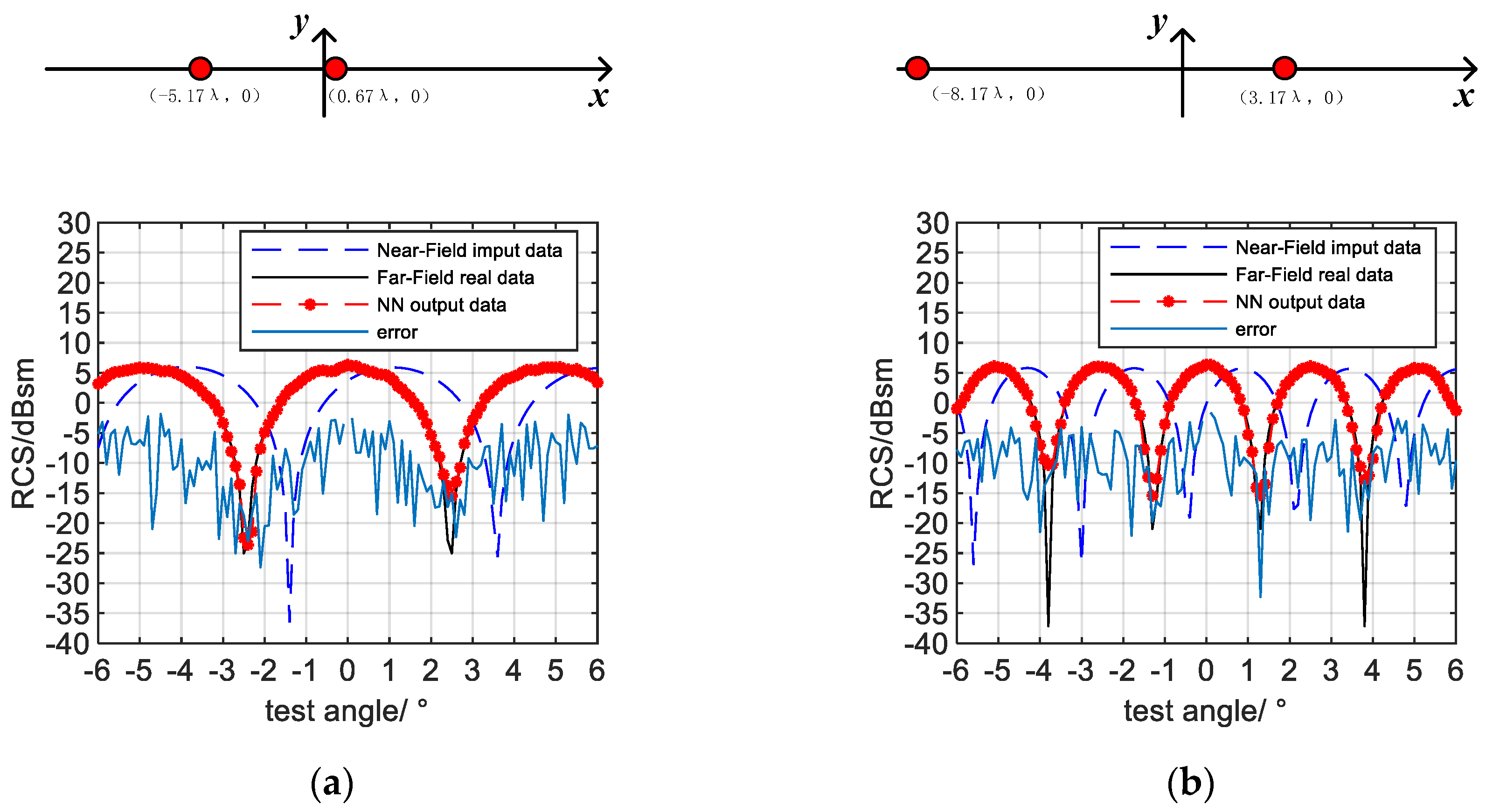
3.2. Comparison
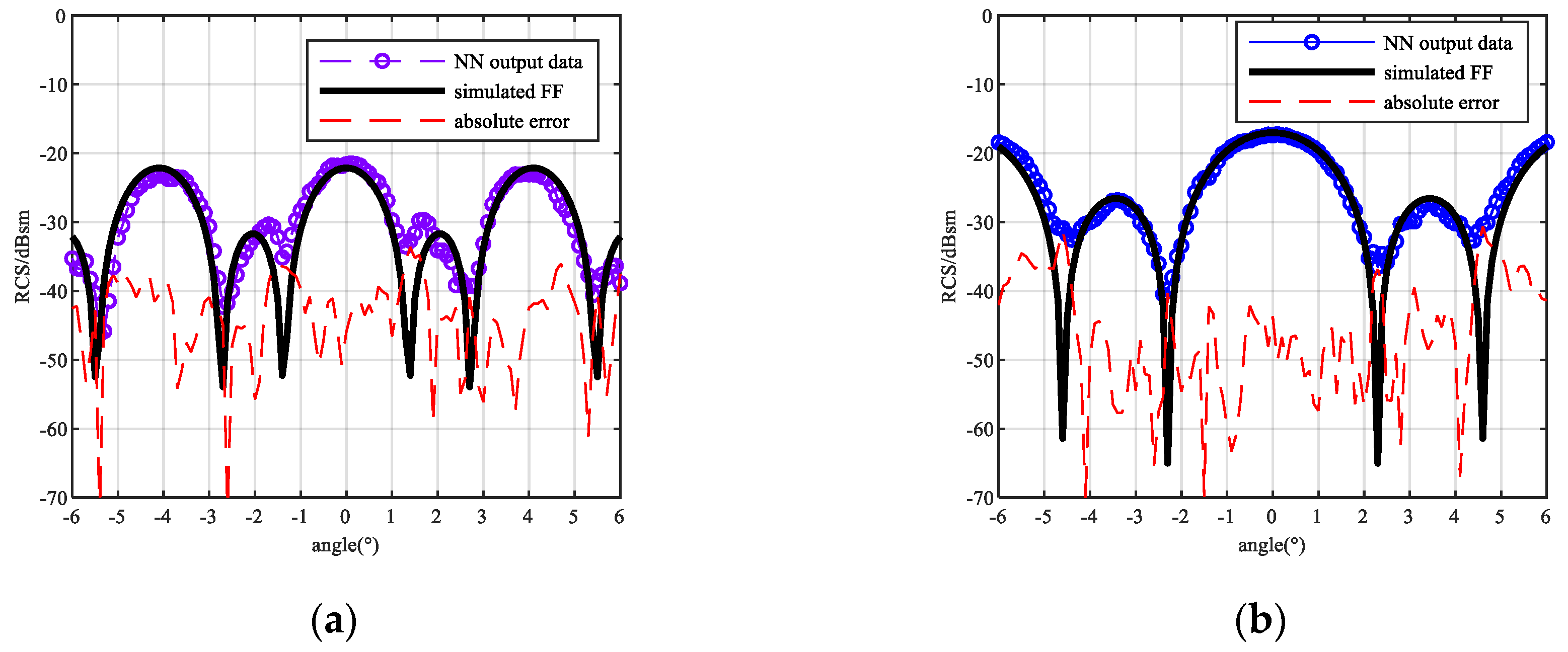
3.3. Performance
3.4. Run Time
3.5. Flexibility
4. Real Scene Experiment
4.1. Experiment Setup
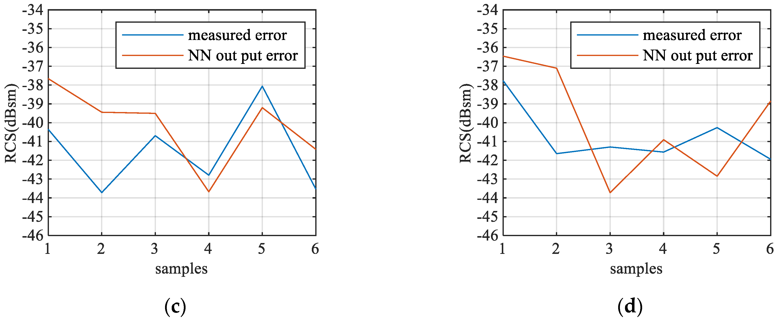
4.2. Result and Discussion
5. Conclusions
Author Contributions
Funding
Acknowledgments
Conflicts of Interest
References
- Knott, E.F. Radar Cross Section Measurements; Springer Science & Business Media: Berlin/Heidelberg, Germany, 2012. [Google Scholar]
- Ruck, G.T.; Barrick, D.E.; Stuart, W.D.; Krichbaum, C.K. Radar Cross Section Handbook; Plenum Press: New York, NY, USA, 1970; Volume 1–2. [Google Scholar]
- Vaupel, T.; Eibert, T.F. Comparison and Application of Near-Field ISAR Imaging Techniques for Far-Field Radar Cross Section Determination. IEEE Trans. Antennas Propag. 2006, 54, 144–151. [Google Scholar] [CrossRef]
- Osipov, A.; Kobayashi, H.; Suzuki, H. An Improved Image-Based Circular Near-Field-to-Far-Field Transformation. IEEE Trans. Antennas Propag. 2013, 61, 989–993. [Google Scholar] [CrossRef]
- Nicholson, K.J.; Wang, C.H. Improved Near-Field Radar Cross-Section Measurement Technique. IEEE Antennas Wirel. Propag. Lett. 2009, 8, 1103–1106. [Google Scholar] [CrossRef]
- Broquetas, A.; Palau, J.; Jofre, L.; Cardama, A. Spherical wave near-field imaging and radar cross-section measurement. IEEE Trans. Antennas Propag. 1998, 46, 730–735. [Google Scholar] [CrossRef] [Green Version]
- LaHaie, I.J. An improved version of the circular near field-to-far field transformation (CNFFFT). In Proceedings of the 27th Annual Meeting of the Antenna Measurement Techniques Association (AMTA ‘05), Newport, RI, USA, 30 October–4 November 2005; pp. 196–201. [Google Scholar]
- Li, N.; Hu, C.; Li, Y.; Zhang, L. A new algorithm about transforming from near-field to far-field of radar target scattering. In Proceedings of the 2008 8th International Symposium on Antennas, Propagation and EM Theory, Kunming, China, 2–5 November 2008; pp. 661–663. [Google Scholar]
- Lahaie, I.J. Overview of an Image-Based Technique for Predicting Far-Field Radar Cross Section from Near-Field Measurements. IEEE Antennas Propag. Mag. 2003, 45, 159–169. [Google Scholar] [CrossRef]
- Rice, S.A.; LaHaie, I.J. A partial rotation formulation of the circular near-field-to-far-field transformation (CNFFFT). IEEE Antennas Propag. Mag. 2007, 49, 209–214. [Google Scholar] [CrossRef]
- Wei, G.; Yuan, W.; Gao, F.; Cui, X. An accurate monostatic RCS measurement method based on the extrapolation technique. In Proceedings of the 2017 IEEE 9th International Conference on Communication Software and Networks (ICCSN), Guangzhou, China, 6–8 May 2017; pp. 784–788. [Google Scholar]
- Schnattinger, G.; Mauermayer, R.A.M.; Eibert, T.F. Monostatic Radar Cross Section Near-Field Far-Field Transformations by Multilevel Plane-Wave Decomposition. IEEE Trans. Antennas Propag. 2014, 62, 4259–4268. [Google Scholar] [CrossRef]
- Omi, S.; Uno, T.; Arima, T.; Fujii, T.; Kushiyama, Y. Near-Field Far-Field Transformation Utilizing 2-D Plane-Wave Expansion for Monostatic RCS Extrapolation. IEEE Antennas Wirel. Propag. Lett. 2016, 15, 1971–1974. [Google Scholar] [CrossRef]
- Jin, J.-M. Theory and Computation of Electromagnetic Fields; John Wiley & Sons: Hoboken, NJ, USA, 2011. [Google Scholar]
- Seber, G.A.W.; Wild, C.J. Nonlinear Regression; Wiley-Interscience: Hoboken, NJ, USA, 2003; Volume 62, p. 63. [Google Scholar]
- Haykin, S. Neural Networks: A Comprehensive Foundation; Prentice Hall PTR: Upper Saddle River, NJ, USA, 1994. [Google Scholar]
- Ayestarán, R.G.; Las-Heras, F. Near Field to Far Field Transformation Using Neural Networks and Source Reconstruction. J. Electromagn. Waves Appl. 2012, 20, 2201–2213. [Google Scholar] [CrossRef]
- Goodfellow, I.; Bengio, Y.; Courville, A. Deep Learning; The MIT Press: Cambridge, MA, USA, 2016. [Google Scholar]
- Dong, C.; Loy, C.C.; He, K.; Tang, X. Learning a Deep Convolutional Network for Image Super-Resolution. In Proceedings of the 13th European Conference on Computer Vision, ECCV 2014, Zurich, Switzerland, 6–12 September 2014. [Google Scholar]
- Weidong, H.; Wenlong, Z.; Shi, C.; Xin, L.; Dawei, A.; Leo, L. A Deconvolution Technology of Microwave Radiometer Data Using Convolutional Neural Networks. Remote Sens. 2018, 10, 275. [Google Scholar]
- Lim, B.; Son, S.; Kim, H.; Nah, S.; Lee, K.M. Enhanced Deep Residual Networks for Single Image Super-Resolution. In Proceedings of the 2017 IEEE Conference on Computer Vision and Pattern Recognition Workshops (CVPRW), Honolulu, HI, USA, 21–26 July 2017. [Google Scholar]
- Hu, W.; Li, Y.; Zhang, W.; Chen, S.; Lv, X.; Ligthart, L. Spatial Resolution Enhancement of Satellite Microwave Radiometer Data with Deep Residual Convolutional Neural Network. Remote Sens. 2019, 11, 771. [Google Scholar] [CrossRef] [Green Version]
- Ledig, C.; Theis, L.; Huszar, F.; Caballero, J.; Aitken, A.; Tejani, A.; Totz, J.; Wang, Z.; Shi, W. Photo-Realistic Single Image Super-Resolution Using a Generative Adversarial Network. arXiv 2016, arXiv:1609.04802. [Google Scholar]
- Bhalla, R.; Ling, H. Near-field signature prediction using far-field scattering centers extracted from the shooting and bouncing ray technique. IEEE Trans. Antennas Propag. 2000, 48, 337–338. [Google Scholar] [CrossRef]
- Swerling, P. Radar probability of detection for some additional fluctuating target cases. IEEE Trans. Aerosp. Electron. Syst. 1997, 33, 698–709. [Google Scholar] [CrossRef]
- Swerling, P. Probability of detection for fluctuating targets. IRE Trans. Inf. Theory 1960, 6, 269–308. [Google Scholar] [CrossRef]
- Lo, Y.T.; Lee, S.W. Antenna Handbook; Springer: New York, NY, USA, 1988. [Google Scholar]
- Vieira, D.A.G.; Travassos, L.; Saldanha, R.R.; Palade, V. Signal denoising in engineering problems through the minimum gradient method. Neurocomputing 2009, 72, 2270–2275. [Google Scholar] [CrossRef]


| Framework | Pre-Preparation Time 1 | Operation Time | RMSE | Experiment Data Acquisition Time 2 |
|---|---|---|---|---|
| NN-NFFFT | 275 s | 0.289 s | −10.28 dBsm | 12 s |
| “image-based” NFFFT | none | 5.568 s | −6.748 dBsm | 244.5 s |
| Sample Number | Metal Sphere Diameter | Project Area of the Sphere | NRCS 1 a at 10 GHz | RCS |
|---|---|---|---|---|
| 1 | 45 mm | −27.987 dBsm | 1.427 dB | −26.557 dBsm |
| 2 | 25 mm | −33.092 dBsm | 1.433 dB | −31.665 dBsm |
Publisher’s Note: MDPI stays neutral with regard to jurisdictional claims in published maps and institutional affiliations. |
© 2020 by the authors. Licensee MDPI, Basel, Switzerland. This article is an open access article distributed under the terms and conditions of the Creative Commons Attribution (CC BY) license (http://creativecommons.org/licenses/by/4.0/).
Share and Cite
Liu, Y.; Hu, W.; Zhang, W.; Sun, J.; Xing, B.; Ligthart, L. Radar Cross Section Near-Field to Far-Field Prediction for Isotropic-Point Scattering Target Based on Regression Estimation. Sensors 2020, 20, 6023. https://doi.org/10.3390/s20216023
Liu Y, Hu W, Zhang W, Sun J, Xing B, Ligthart L. Radar Cross Section Near-Field to Far-Field Prediction for Isotropic-Point Scattering Target Based on Regression Estimation. Sensors. 2020; 20(21):6023. https://doi.org/10.3390/s20216023
Chicago/Turabian StyleLiu, Yang, Weidong Hu, Wenlong Zhang, Jianhang Sun, Baige Xing, and Leo Ligthart. 2020. "Radar Cross Section Near-Field to Far-Field Prediction for Isotropic-Point Scattering Target Based on Regression Estimation" Sensors 20, no. 21: 6023. https://doi.org/10.3390/s20216023