The Possibility of Using the Chapman–Richards and Näslund Functions to Model Height–Diameter Relationships in Hemiboreal Old-Growth Forest in Estonia

Abstract

In light of the difficulties in stand volume estimation of natural forests, we analyzed height–diameter relationships and derived a set of height estimation equations for volume estimation for naturally developing forest ecosystems, using the Järvselja old-growth and the Laeva commercial forest in Estonia as a case study. This contribution presents an approach to model individual tree height–diameter relationships for Scots pine, common aspen, silver and downy birch, Norway spruce, black alder, gray alder, linden species, European ash, Norway maple, deciduous species and coniferous species in multi-size and mixed-species naturally developing stands in Estonia. Single-tree-level data were collected in 2013. Two methods were used to obtain stand-level data: whole surface inventory and partial surface inventory. To model the height–diameter relationship in naturally developed mixed-species forest stands in order to predict single tree height based on observed diameter at breast height, we applied nonlinear mixed models where we applied the Chapman–Richards and Näslund models as fixed-effects and the influence of the species contribution at the sites as random effects. The fixed-effects followed a set of criteria: (1) height starts at h = 1.3; d = 0; (2) the applied functions are monotonically increasing with a clear inflection point and 3) the fixed-effect model has an asymptotic value) in a naturally developed mixed-species forest.

1. Introduction

The accurate estimation of biomass is an important task in forest ecosystem management planning and pivotal to conduct resource risk impact assessments. The classical approach establishes an appropriate relationship between the tree height (H) and its diameter (D) (i.e., H-D functions) at the tree stand or tree species level [1,2]. Since the initial data used to develop H-D functions are often developed based on single species managed forests and have temporal and spatial limitations, the suitability of the developed functions should be tested when fitting models to the existing data. Nevertheless, caution should be taken when considering the growth of trees that developed under different disturbance regimes or under management conditions [3,4]. Our knowledge of the allometry linking a tree’s diameter at breast height (DBH) and its total height is a fundamental feature for assessing the stand or tree volume and applying different growth and yield models for resource planning. Although DBH is easily obtained, either for all trees or for selected trees measured on a sample plot, the height measurements are notoriously time-consuming and in some cases, stand conditions make it difficult or impossible to establish them [5,6]. This usually results in a sub-sample of tree heights measured across the range of diameters observed on a site [5,7]. A large share of existing H-D models is based on single species dominated cultivated stands [1,2] and are therefore describing different tree allometry as in the case of multi-species naturally developing stands [3,4]. Some former studies suggest that the H-D allometry is needed to be described and modeled separately on stands with natural or anthropogenic disturbances [5,6,7]. Today, the use of remotely sensed data in forest inventories has created an urgent need for H-D data, especially at places where the distribution of tree heights needs to be related to DBH. Today, the wider use of the combination of remotely acquired height data in combination with ground measurements has become a standard analysis tool for forest resource assessment. These data have considerable influence on all height distribution-dependent response variables like mean height, standing volume, etc. [8].

The H-D relationship is largely species-specific and depends on the stands’ structural features [9,10], the stand development history [11,12] and the prevailing disturbance regime [9,12]. The H-D relationship could be studied at the stand or individual tree level. Stand related functions are often more robust and simpler than the more complex individual-tree-related functions that use tree characteristics [13]. Until today, the H-D relationship was most frequently used for estimating the merchantable wood in stand by average tree volume [14]. In this case, the focus has been on the allocation of round wood products such as poles for fences, sawn wood, pulp and paper, and plywood and very often, the desired accuracy of the assortment distribution has guided the modeling effort [14]. Nowadays, inventories of forest resources aim to quantify ecosystem services such as carbon sequestration, biodiversity conservation and water storage and purification properties, in addition to forest management and timber assessment [15]. Still, the size and volume related estimations in ecosystem services include very often H-D relationship as calculation proxy.

There are some studies and applications of the H-D relationship available that are applied in the Estonian context. Padari [16,17], for example, proposed an H-D function at the individual tree level for various species that were dependent on D as a predictor for estimating H, without considering other stand variables for managed forest conditions. Nilson [18] included the mean height and the quadratic mean diameter of trees within stands in his function. Padari et al. [7] analyzed the dominant tree selection method for stand mean height modeling in young naturally regenerated stands. Schmidt et al. [19] modeled the H–D relationship as a function of only the stand quadratic mean diameter (Dg) and the plot’s geographical coordinates using the Estonian Network of Forest Research Plots. Kiviste and Kiviste [20] presented different equations of stand height depending on stand age and site factors. Kängsepp et al. [21] analyzed the Weibull distribution function as the fit function for empirical height distributions of young naturally developing forest stands in consecutive years and found that the Weibull’s distribution shape parameter was related to the maximum height and height range, while the scale parameter was related to the mean, quadratic mean and median heights. Motallebi and Kangur [6] reported an increasing trend of the slenderness of Scots pine (Pinus sylvestris L.), which reached a peak and then continued with a decreasing trend towards the end of a tree’s.

The aim of our study was to describe and analyze single tree growth allometry through the H-D ratio in the stand composition that was formed in natural conditions. With the current study, we aim to provide a tree species-specific H-D model calibrated on mixed-species multicohort stands to be used to model the single tree height and diameter in old-growth forest assessment.

2. Materials and Methods

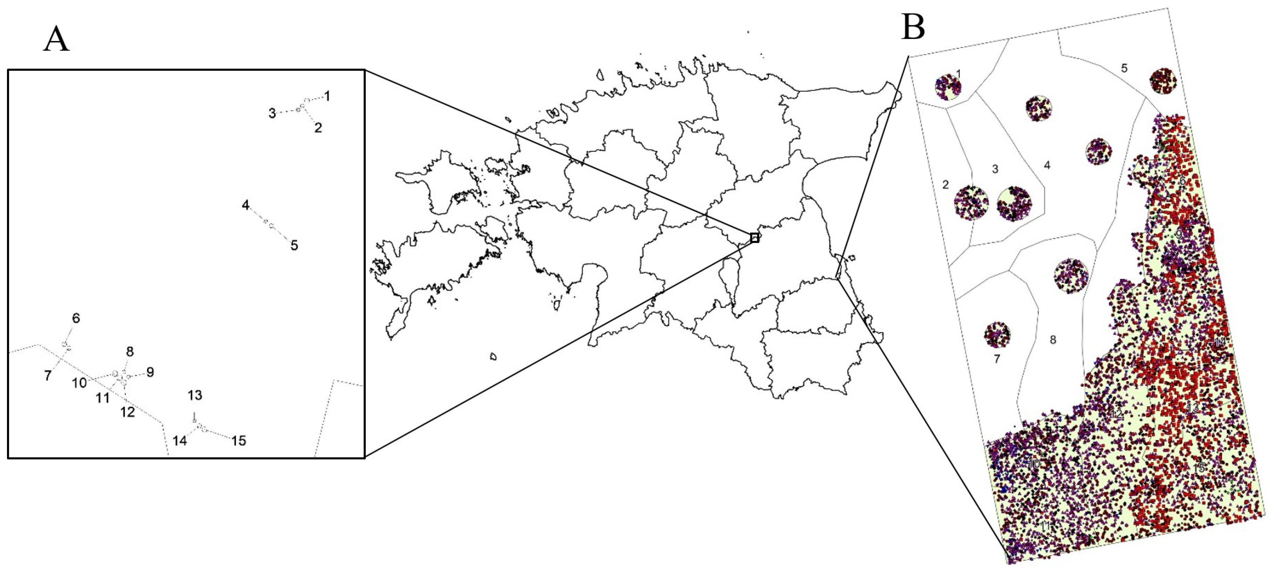
2.1. Description of the Study Site

The study area is located in Järvselja Training and Experimental Forest Centre that is part of the Järvselja nature protection area established in 1924. Today, the old-growth forest compartment and its surrounding compartments are part of the Järvselja nature protection area that covers more than 174 ha. According to the site protection plan, this area is divided into two special management zones (Ürgmets and Järvselja) and one partially limited management zone (Apna) [22].

The protected old-growth forest compartment (known as JS226) [22,23] is the most important and scientifically interesting and also the most studied area in the nature reserve (see location on Figure 1.). It is divided into 15 sub-compartments, which altogether cover 19.7 ha according to the 2010 stand-wise forest inventory. There are three different Natura 2000 habitat types located in this compartment: 91D0 (bog woodlands), 9020 (Fennoscandian hemiboreal natural old broad-leaved deciduous forests) and 9050 (Fennoscandian herb-rich forests with Norway spruce (Picea abies (L.) H.Karst.)). There are several protected habitats in the compartment for the following species: Epipactis helleborine (L.) Crantz, Skeletocutis odora (Peck ex Sacc.) Ginns, Cypripedium calceolus L., Cinna latifolia (Trevir.) Griseb., Corallorhiza trifida Châtel., Corydalis intermedia (L.) Mérat, Amylocystis lapponica (Romell) Singer, Leucopaxillus salmonifolius M.M. Moser & Lamoure, and Tricholoma apium Jul. Schäff.

Compartment JS226 (58°16′42″ N and 27°19′28″ E) is divided among three dominating vegetation types (by Lõhmus [24]): on the eastern side, fresh boreo-nemoral forests with rich groundcover species like Oxalis acetosella L., Hepatica nobilis Schreb., Rubus saxatilis L. and Maianthemum bifolium (L.) F.W.Schmidt. The western side is dominated by drained mixotrophic bog forests, dominated by Scots pine (Pinus sylvestris L.) and Norway spruce in the tree layer. The middle of the compartment is a fen, with a constantly high groundwater table and with a very luscious plant cover. Dominant tree species are black alder (Alnus glutinosa (L.) Gaertn.) and silver birch (Betula pendula Roth).

To allow a comparison with a managed and even-aged stand type, we used data of the Estonian Network of Forest Research Plots (ENFRP) [25]. For comparison, plots describing old stand conditions (average age of dominating species ranging between 80 and 100 years) in naturally established stands (naturally regenerated after World War I), and later in managed stands in central Estonia in the Laeva municipality (58°32′22″ N and 26°23′44″ E) growing on a fresh boreo-nemoral forest type (Figure 1.). This resulted in a dataset of 15 plots dominated by silver birch and common aspen (Populus tremula L.). As is common on these fresh fertile sites, shade-tolerant species like Norway spruce and/or small-leaved lime (Tillia cordata Mill.) form a stable secondary cohort in all plots. These plots represent stands growing on historic state lands and have a management history following the best silvicultural practice in the area. Data from the last measurement in 2015 were used.

2.2. Data Collection

From spring 2013 until autumn of the same year, an inventory was carried out to cover the study area with tree mapping data. To avoid potentially disruptive extensive measurements on fragile sites and close to habitats under protection, two methodologies were followed: whole surface inventory (in sub-compartments 6, 9, 10, 11, 12, 13, 14, 15) and partial surface mapping based on permanent sample plots (in sub-compartments 1, 2, 3, 4, 5, 7, 8). The whole surface mapping covered 9.34 ha, and the partial mapping covered 10.03 ha. The study area covered five different site types: Oxalis-drained peatland site type 1.52 ha, minerotrophic mobile water swamp forest site type 2.31 ha, Vaccinium myrtillus-drained peatland site type 6.07 ha, Aegopodium site type 6.62 ha and mixotrophic bog forest site type 2.84 ha (forest site types described following the Lõhmus 2004 forest site type typology [26]).

We applied the Field-Map technology (IFER-Monitoring and Mapping Solutions Ltd., Jílové u Prahy, Czech Republic) in conjunction with geodetically accurate reference points (data not presented here), where the distance between trees was measured with ForestPro impulse laser rangefinder. For tree positioning, the Mapstar TruAngle angle encoder together with ForestPro impulse laser rangefinder was used. Tree heights of the live crown base and heights of the dry branch base were measured with a Vertex hypsometer to the nearest 0.1 m. Data were collected and stored on-site with the FIELDMAP data collector software. Partial surface stem mapping was carried out in parallel with full surface stem mapping on wetter and more fragile sites. Circular plots of various radii (15–20 m) were used in different sub-compartments. Permanent plots were located similarly with Field-Map measurements using the geodetically accurate reference points (see Figure 1.)

Both full surface and partial surface tree mapping followed the design of the survey protocol by the Estonian Network of Forest Research Plots [25,27]. For live standing trees, all trees with DBH larger than 7 cm were measured. For every tree, measurements included tree position, tree species, tree height, live crown length, and diameter (in two perpendicular directions). In the case of full surface tree mapping, tree height was recorded for all measured trees. The tree layer was divided according to tree classes into the upper story (dominant layer and secondary cohort) and lower story (understory cohort and regeneration layer).

More than 7,000 live trees, snags, standing dead trees—7,000 in the Järvselja and 2,000 and in the Laeva sites (see

Table 1. Summary statistics of the measured data.

Variable	Live Trees		Standing Dead Wood		Snags		Downed Dead Wood
	Järvselja	Laeva	Järvselja	Laeva	Järvselja	Laeva	Järvselja	Laeva
Number of measured, (N)	6008	1702	263	256	1097	188	2983	116
Number estimated trees per compartment	15,480	-	1060	-	2661	-	6112	-
Dominating species *	SP, LI, BAR, BI, NOM	SP, BI, CA, LI	SP, LI, SP	SP, BI, CA	SP, SP, AH	SP, BI, CA	BI, SP, BAR, LI,	SP, BI
Mean diameter, D (cm)	19.0	27.3	19.6	24.0	26.9	22.6	25.1	17.9
Mean height/length, H/L (m)	17.3	25.6	8.1	25.4	4.4	6.6	8.6	16.9

* tree species codes are as follows: BI = birch (silver birch and downy birch (Betula pubescens Ehrh.)); NS = Norway spruce; BAR = black alder; SP = Scots pine; LI = lime family; AH = European ash (Fraxinus excelsior L.); NOM = Norway maple (Acer platanoides L.); CA = common aspen.

)—were used in this study. The most common tree species in all woody cohorts were Norway spruce and lime.

2.3. Model Type Selection to Describe the H-D Relationship in Naturally Developing Forest

Many different growth models that describe allometric relations in tree growth are used on a regular basis in forest management. We can roughly distinguish two classes of models. One class that may be used because it is known to produce robust fits to data, but the mathematical relation applied does not stem from an understanding of the process [28]. The other class of models stems typically from a process or mechanistic understanding of the growth process, and the parameters of the models have a physiological meaning [2].

One class of models descends from the von Bertalanffy growth model [29] and is rooted in a systems theoretical approach. The structure of these models usually includes a growth term and a limiting term, leading to either a convex or an S-shaped curve. We used the Chapman–Richards function [30], which has been applied in forest growth and yield estimations [31,32]. The model describes the tree height h in relation to the diameter d at breast height (Equation (1)):

$$\frac{dh}{dd}=\alpha h^m-\beta h,$$

(1)

where the parameters α and m are linked with the growth dynamics of height and β with the limitations on height growth. Because models of this type have their origin in a scaling law [29], they are not limited to specific age classes as they usually occur in managed forest stands. We do not discuss the deduction of the parameters here further and note that for fitting the model to data the integrated form (Equation (2)):

$$h\left(d\right)=h_{of}+ h_{mx} {\left(1-e^{-kd}\right)}^p,$$

(2)

was used. The parameters h_mx (maximal height), k (growth dynamics), and p (empirical parameter linked to catabolism that is proportional to the organism’s size) are determined by nonlinear regression to the data. The offset parameter h_of is set to 1.3 m to account for the height where diameter usually is measured.

There are numerous model shapes and approaches used to describe the height curve in the same age and multi-age stands [33]. We implemented Chapman’s and Näslund’s model equations as representatives that are used commonly in managed forests for growth and yield estimations.

2.4. Modeling of H-D Relationship

To assess the height–diameter relationship of old-growth hemiboreal forests, we used a nonlinear mixed-effects model approach. For H-D relationships, the species was a naturally occurring grouping or clustering factor. For the fixed-effects nonlinear models, Chapman–Richards and Näslund equations were applied, and, consequently, the tree species was chosen as a random effect. We used the nlme R package [34] for the calculations.

To parameterize the fixed-effects of the Chapman–Richards function, we used nonlinear regression with initial guesses on the parameters. The offset h_of was chosen as a constant (1.3 m) and was not subject to the regression itself. Our prior knowledge about the height of the forest let us estimate the initial value of the maximal height h_mx to be near the average height measured for the largest diameters as it denotes the asymptotic value if the diameter grows towards infinity ($d\to \infty$). The growth dynamic (slope and inflection point) of Equation (2) is determined by the parameters k and p for typical H-D relations; the range for this parameter lies below 0.05 cm⁻¹. We set the initial value here to 0.1 cm⁻¹, which turned out to be near enough to allow proper fitting. However, the empirical parameter p modulates the curvature of the model, and it also impacts the slope and the inflection point. Typical values for p are above 1, and because the growth in stem diameter is proportional to the volume of water that is evaporated [35,36], we used a scale value that is between the dimension of an area and of a volume and initially set this parameter to 2.5.

In a similar approach, the Näslund function’s parameters were estimated as fixed-effects. From our prior knowledge on equation 3 and by choosing a controlled starting point (1.3 m), the function is known to ascend when a > 0 and it converges towards the asymptote $h_{mx}=1.3+{\left(\frac{1}{b}\right)}^3$ [19,37]:

$$h\left(d\right)=1.3+{\left(\frac{d}{a+b·d}\right)}^3$$

(3)

where h refers to tree height, d is the diameter at breast height (DBH), a and b are model parameters. To allow direct comparison between both models, asymptotic height predicted, we rescaled the parameter $b= \sqrt[3]{1/\left(h_{mx}-1.3\right)}$. Initial values chosen were a = 1 and h_mx = 40, which produced good fits for all species or plots.

To assess the D-H relationships, we removed tree species from the analysis where only a few measurements were recorded, or the species occurred under the canopy only. Sometimes these were single measurement points or the sample size was too small to allow a proper fitting of the fixed model. In the case of the old-growth forest stands in Järvselja, from all of the 17 reported species, the seven tree species that remained in the analysis were birch, spruce, black alder, aspen, pine, lime, and maple. We tested the model as well on all species, but in the case of measurements below 12–15 readings, the fixed model failed to provide parameters, and the result of the mixed-effect models was not changed. In the managed forest stands in Laeva altogether, 8 species were measured. Here, we also removed the understory species and those with a small number of measurements. The species used for the H-D relationships that remained were birch, common aspen, Norway spruce, lime, and gray alder (Alnus incana (L.) Moench).

Depending on the number of parameters of the fixed model, we employed the random factor to set up different models to test with the data. For the Chapman model, three models were calculated, and we let the tree species as random effect influence one (CA1h), two (CA2hp) or all three (CA3hkp) parameters. These were chosen from the set of a total of 7 possible combinations that include random effects of the Chapman model. In the case of the Näslund equation, the two parameters of the fixed-effects model allowed for two different mixed models, out of possible three, where the random effects influenced either one (NA1b) or both (NA2ab) parameters. The choice of parameter combinations was due to the prior knowledge that naturally developing stands have a higher variation in height growth [7,11,14,20]. Altogether, by this, we achieved five models that were fitted to the data of the unmanaged old-growth forest in Järvselja and the managed forest in Laeva.

For each dataset, we assessed the models AIC [38] as a criterion to decide which of the models performed best. However, we hasten to say that it is not possible to compare in this way between two different datasets or sites and therefore, the model performance can be compared only within one dataset.

2.5. Comparative Analysis of H-D Modeling Results

For relationship comparisons, H-D scatterplots for the main tree species were compiled and then added H-D curves from the Järvselja old-growth forest. Finally, an H-D relationship empirical smoother [39] with 95% of the confidence interval of the mean was added.

We checked for all models the standard criteria, normality of residuals and constant variance of the residuals. Applying the constant error model with the assumption that the errors are Gaussian random variables was matched in all cases (see Figures S1 and S2, Tables S1 and S2 in the supplementary material).

3. Results

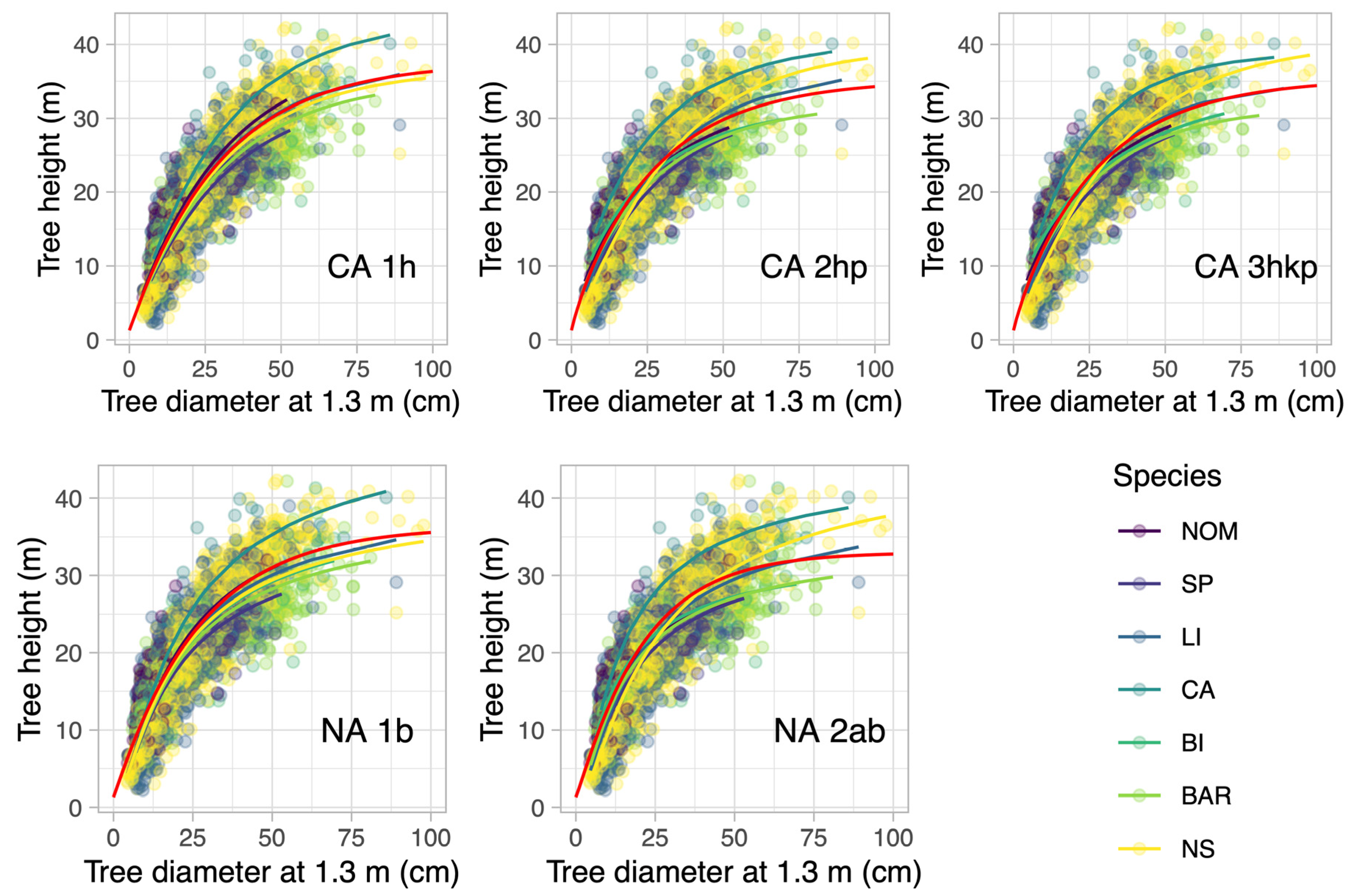
3.1. Modeling Results of the Old Growth Forest

For the old-growth forest in Järvselja, the nlme model estimated overall an asymptotic height of 34.1 m in the case of the best-fit model CA3hkp according to the AIC criterion (see

Table 2. Akaike’s information criterion (AIC) and coefficients for the modeled height–diameter (H-D) relationships. Chapman–Richards models (CA) 1–3 and Näslund models (NA) 1–2 describe the different levels of influence of the random effect “species” on the parameters of the fixed-effect models. Parameters are given as value ± standard deviation. Details on the random effects are given in the supplemental material.

Location	Equation	AIC	hmx	k	p	a	hmx
Järvselja	CA 1h	26,515.46	36.27 ± 1.26	0.034 ± 0.002	1.027 ± 0.024	-	-
	CA 2hp	25,974.98	33.89 ± 1.41	0.035 ± 0.002	0.900 ± 0.064	-	-
	CA 3hkp	25,974.84	34.06 ± 1.43	0.035 ± 0.004	0.911 ± 0.075	-	-
	NA 1b	26,662.17	-	-	-	1.794 ± 0.015	42.09 ± 1.54
	NA 2ab	26,089.33	-	-	-	1.519 ± 0.123	38.57 ± 2.02
Laeva	CA 1h	2300.34	32.96 ± 1.78	0.085 ± 0.005	1.898 ± 0143	-	-
	CA 2hp	2232.85	38.43 ± 0.65	0.046 ± 0.003	1.070 ± 0.157	-	-
	CA 3hkp	2234.85	38.43 ± 0.65	0.046 ± 0.003	1.069 ± 0.157	-	-
	NA 1b	2352.55	-	-	-	1.514 ± 0.052	46.33 ± 2.90
	NA 2ab	2243.96	-	-	-	1.454 ± 0.0206	46.06 ± 1.70

). Depending on the models, the predicted asymptotic heights ranged between 33.9 m for CA2hp and 42.1 m for NA1b. The height estimates of the Chapman models were lower (33.9–36.3 m) than the estimations of the Näslund models (38.6–42.1 m). Overall, the models where the random factor was allowed to influence all parameters showed better results in estimating the H-D relationship (Figure 2). That statement holds according to our results for the estimation of the clustered data (species wise) and the overall estimation. It is further notable that for the dataset obtained from the old-growth forest in Järvselja, the fixed-effect Chapman–Richards model alone did not manage to obtain parameters for pine and birch species clusters. While the nlme models obtained valid estimators for all species, it can be seen in Figure 2 that while using the model CA1h, the single random influence on the parameter h_mx captures the variety in all H-D relationships already well. Adding more random influences to the parameter p as seen in Figure 2 CA2hp and finally, on all parameters, CA3hkp is consolidating the height estimation of the overall relationship towards a height of 34 m. The major variation occurred in height, and therefore, the location of the growth curves inflection points remained rather fixed. Letting the random factor influence two parameters (CA2hp) increased the species variability, but still, the models headed towards a common, now the lower asymptotic height of 33.9 m and especially the estimated asymptotic height of Norway spruce increased while lime trees asymptotic height was slightly reduced. In the case where all three parameters of the Chapman–Richards model was influenced by the random factor (CA3hkp), the species-wise models showed the largest variability in height estimations, which, however, led to an estimation of the H-D relationships asymptotic height of 34.05 m.

In comparison, the commonly used Näslund equation offers two possible parameters for the variation by the random factor. Starting with the parameter b, which determines the asymptotic height, the NA1b model estimates a height of 42.1 m and already shows large variability in the individual H-D relationships per species. Adding the parameter a to the random variation (NA2ab) led to an estimation of the asymptotic height of 38.6 m. That parameter determined the location of the curve’s inflection point; its variation improved the mapping of the species clusters data and also led to an increase in the Norway spruce estimation. In comparison with the Chapman–Richards model, the models based on the Näslund equation produced heights that tended to the uppermost estimates.

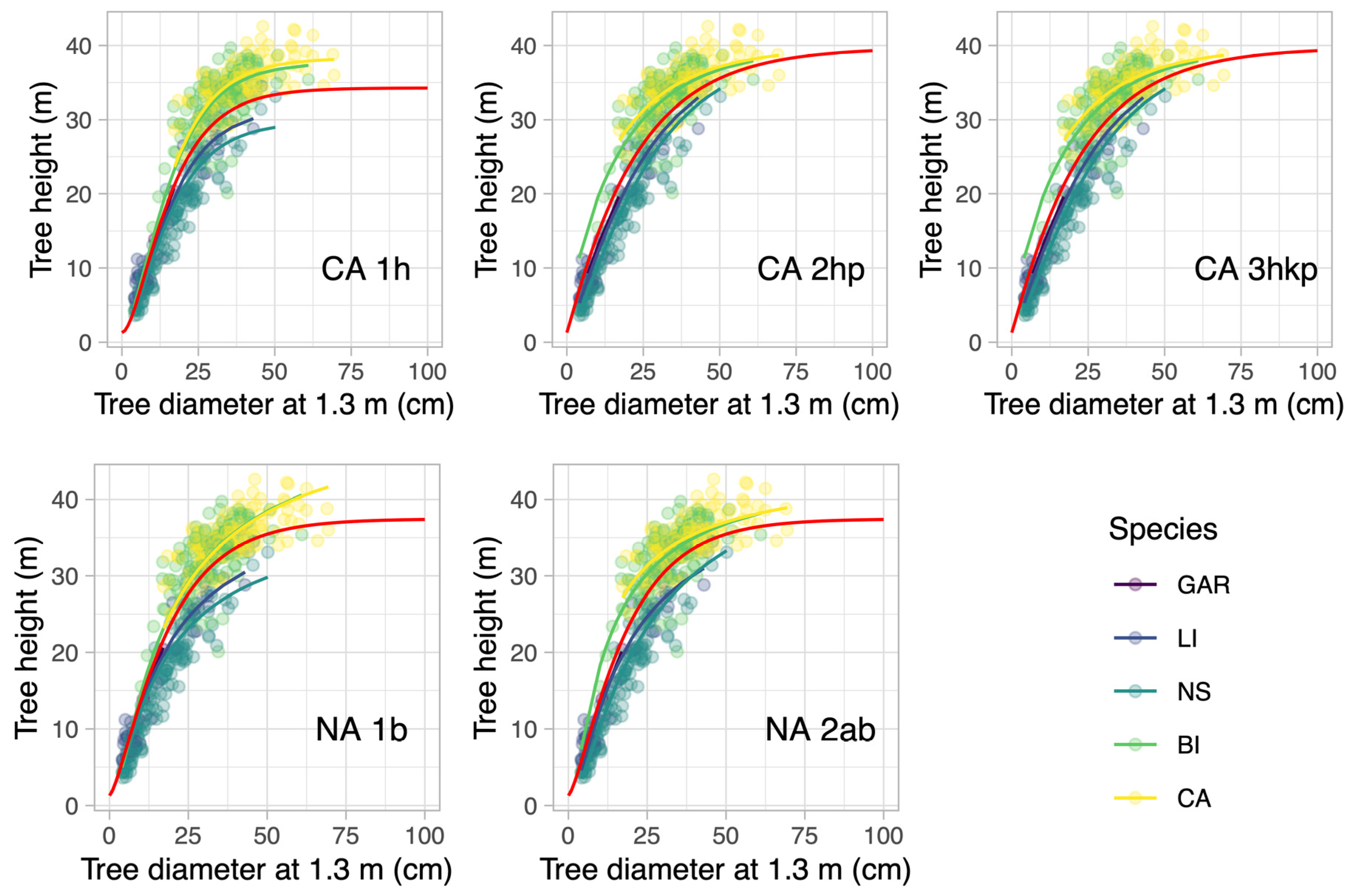
3.2. Modeling Results of the Managed Forest

For the dataset obtained in the managed forest in Laeva (Figure 3), the Chapman–Richards models CA1h produced the lowest height estimate of 33.0 m, but CA2hp and CA3hkp a rather similar estimate of all parameters. The asymptotic height was estimated in all these cases to be 38.4 m. There was also almost no variation in the second parameter (k) and only a very small change in the third parameter (p) for the cases with higher random influences. In the case of the gray alder data, the few data points led to a failure in determining the fixed-effect model parameters, but the mixed-effect models achieved a result. The AIC criterion points to the Chapman–Richards function with all parameters influenced by the random effect of the species to provide the overall best estimation of the data.

The Näslund equations (NA1-2) gave different estimates for the asymptotic height in the range of 46.3 m (NA1b) and 46.1 m (NA2ab) that are quite higher than produced by the Chapman–Richards model ensemble. However, the variation between the species clusters was larger in the case of Näslund models.

3.3. Model Selection and Comparison

The height–diameter relationship was analyzed, and the height curve modeled to predict single tree height based on observed diameter at breast height. Traditionally, H-D curves were set to [19]: (1) start at h = 1.3; d = 0; (2) they are monotonically increasing with a clear inflection point and (3) they reach an asymptotic value [40]. We applied Akaike’s information criterion (AIC) as a model selection criterion that takes the goodness of fit via the likelihood function into account and at the same time sets a penalty on the number of model parameters (see Table 2). In that way, AIC allows selecting the models while avoiding overfitting. The AIC does not allow us to directly compare the two different datasets, but we can determine the model that does fit best within one dataset. For the old-growth forest, CA3hkp obtained the minimal AIC, and for the managed forest, it was CA2hp, but the difference to the model with a random effect of species in all parameters (CA3hkp) was marginally (see Table 2).

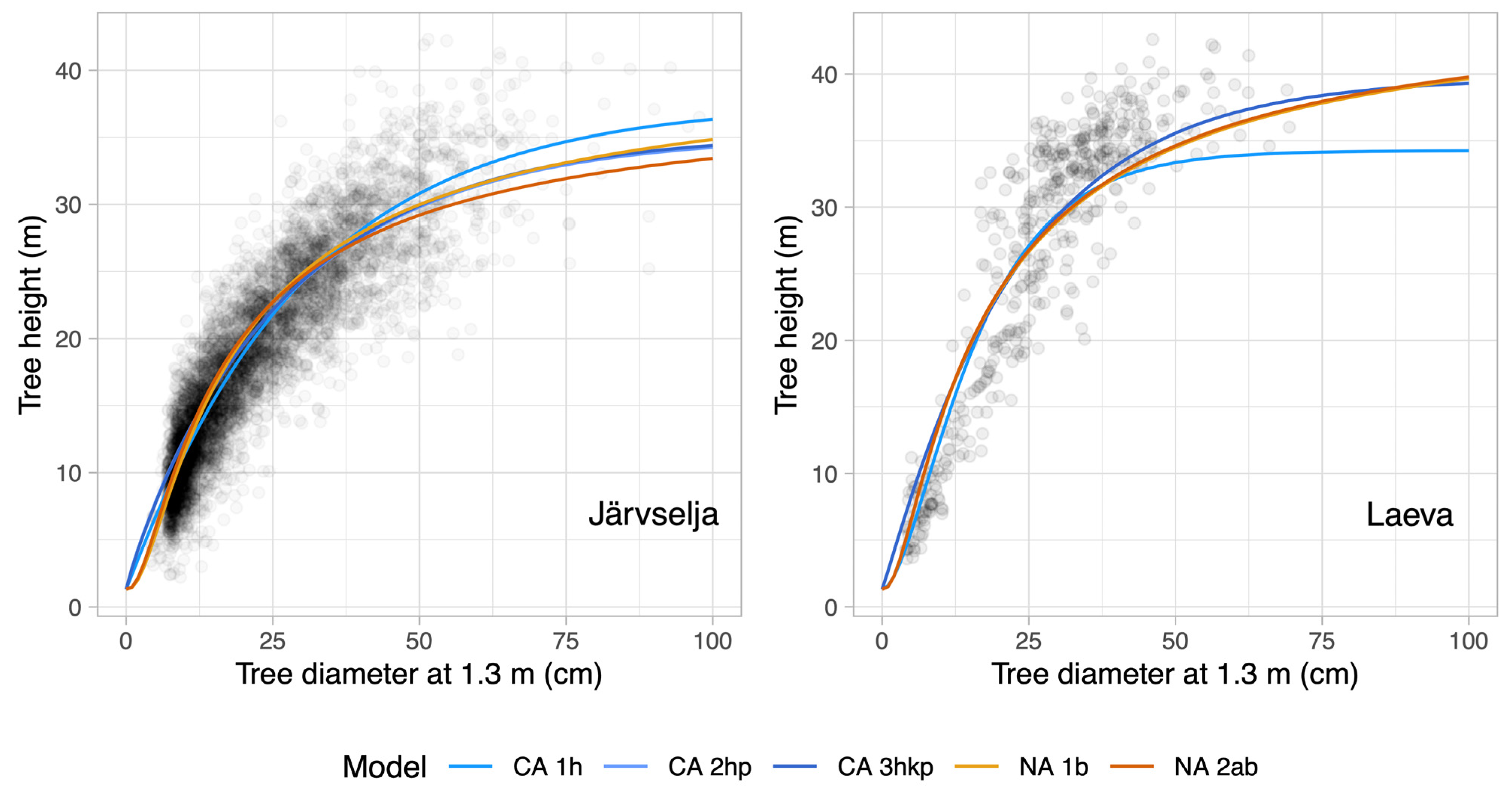
3.4. A Comparison of Old-Growth Height Curve Modeling Results with Managed Forests Height Curves

A comparison of H-D curves modeling based on 404 height and diameter measurements of Norway spruce, silver birch, common aspen and lime trees showed that small trees dominated the results in the old-growth forest.

One feature that is well visible (Figure 2, Figure 3 and Figure 4) is the difference between the number of small trees that dominate the data in the old-growth forest. In the managed forest, the species also had a clearer distinction in height, and clusters were visible. There, spruce and aspen-dominated the higher canopy while the other species remained below. In contrast, in Järvselja, in the old-growth forest, the height range from 10 to 30 m dominates the data.

From Figure 5 clear trends became visible when comparing managed and natural stand conditions. For smaller average diameters (D < 20 cm), there was no clear allometric difference between trees growing in Järvselja old-growth forest and Laeva managed forests. In the case of larger diameter trees (D > 20 cm), the average height in the Laeva managed forests was considerably higher than in Järvselja old-growth forest. Especially large differences occurred when comparing silver birch, but also in the case of common aspen height curves.

4. Discussion

Models like that of Näslund have been developed to estimate the growth and yield of managed forest stands and as a tool for optimization and planning of management activities [1,3]. In natural stands, no optimization on yield is usually done, and a higher heterogeneity according to the diameter to height relationship might be expected [21,41]. The idea of an S-shaped relationship is linked to the biological observation that tree growth follows two processes, one that relates the change in stem volume or diameter increment to the volume or diameter itself and another process that limits the growth by resource availability in relation to the volume or diameter [6]. That leads to a shape with an asymptotic behavior and an inflection point at the point of highest or optimal growth. The Chapman–Richards model follows that approach (Equation (1)) and is widely used in forestry and other scientific fields to describe growth [2,42]. All variations of the models fitted to data (Figure 2, Figure 3 and Figure 4) showed that a sufficient accuracy was achieved in the regression, and fairly good growth estimations were found. The major differences were in the onset of the H-D curves (Figure 4), where no data were available, and to the larger diameters, where the number of data points was less.

The differences between the model estimations, even large ones, in the onset of the growth curves did not impact the goodness of fit because there were no data. In that case, the regression algorithm cannot give any criteria and strictly taken the estimated curve was not valid in that region [43]. Another situation occurred at the end of the curve; there fewer and fewer measurements were available, and therefore, the regression was dominated by the cluster of data with the most measurements. In our case, Norway spruce and lime data had the highest density of measurements at a diameter range between 7 to 30 cm, while birch data were generally scarcer, and the density was higher between diameters 10 to 20 cm. In general, the data clouds we used had a log-normal density distribution in both dimensions, and the estimated growth curves were very similar where the density of measurements was high, but towards the higher diameters, with scarcer data, the estimates differed strongly. While the dispersion in the data carried some information on the stand characteristics, it did not improve the fit. On the contrary, additional measures like constraining the parameter [19] or including a weight function into the fit process may be needed to find appropriate results [18]. Using nonlinear mixed-effect models that included the species as random effect yielded sufficiently accurate estimates of the H-D relationship even in the cases when single species could not reach a parameterization in the fixed-effect model. In his work from 1936 [37], Näslund stated that “a subjective choice of stems” have been made, which is a bit like binning if selected from mean sized trees.

The AIC criteria suggested in all cases that the Chapman–Richards model should be chosen, regardless of the fixed initial height and the differences at the onset that were not captured by the regression algorithm. Because both model ensembles matched well if there were enough measurements, the differences most probably were due to the asymptote with fewer data. Particularly in the case of the old-growth forest in Järvselja, the Chapman–Richards model with random effects on all parameters by the species, the clusters were matched well but showed the largest deviations just in the asymptotic region. Even though Näslund model ensembles had higher AICs, they also showed a larger deviation in the cluster estimates at the asymptote. Because Chapman–Richards uses three parameters while Näslund’s model has two parameters and the resulting estimations did not vary dramatically, no overfitting was apparent. The H-D curves modeling results were fully valid for the current stand composition and developmental stages. In future applications, a parameter estimation will be needed.

Empirical forest growth and yield models depend on the relationship observed between dendrometric variables like tree height and diameter or basal area at breast height. For managed conditions, these models assume constant allometric relationships [2,6]. This is not valid in the case of either long term natural forest dynamics [3,4] or intra- and interspecific variability in trees, relating to changes in stress tolerance and climate-related functional traits [44,45]. In the naturally developing stand conditions, the use of H-D functions has both pros and cons. In the case of the standard analysis of ground-based plot or stand measurements, the use of the H-D relationship is justified, especially when the height and diameter measurements are scarce and do not cover all trees. The use of height curves then avoids irregular and illogical extrapolation. At the same time, the use of two or three-parameter functions may not be flexible enough to describe the full range of the variability in the H-D relations in natural conditions. While under natural conditions, the distribution of the input variable is a more challenging feature, the managed forests have a stronger clustering with a higher distinction of the species clusters according to the diameter. While nlme models achieve a very good estimation on the H-D relation, in both cases, it is visible in Figure 4 for the Laeva data set that the high-density of data between 25 to 50 cm diameter and the cluster below 10 cm diameters do not match well the data right at the inflection point of the growth curves. For this reason, we used height curve assumptions of free numeric smoothing technique in our comparison of Järvselja old-growth and Laeva managed forests.

Short and long-term forest dynamics patterns are related to certain site conditions, tree age and diameter distribution, dominant species, the severity of disturbance, time since last disturbance, and spatial structure in natural boreal forests [4]. The change in the convergence of H-D curves in the case of large-diameter trees in the comparison of Järvselja old-growth forests with the managed forests in Laeva indicated a clear difference in tree allometry due to differences in forest growth and stand demographics. For describing the highly variable allometric condition between trees within the same species in old-growth forests, either the application of constant model parametrization or the application of a more complex approach of allometric plasticity and the introduction of allometric coefficients to the model are required [6].

5. Conclusions

We aimed to describe and analyze growth allometry of the main tree species in stand composition that form in natural conditions in Järvselja old-growth forest in Estonia. We analyzed the species-specific H-D ratio and provided a tree species-specific H-D curve model calibrated under mixed species multicohort conditions. For height curve modeling purposes, we analyzed the performance of two main base functions used for modeling the H-D ratio–Näslund and Chapman–Richards.

Although both model ensembles matched well if there were enough measurements, the AIC criteria suggested in all cases that the Chapman–Richards model should be chosen. The H-D curves modeling results were fully valid for the current stand composition and developmental stages. In future applications, a parameter estimation will be needed.

We carried out a comparison of height curves in Järvselja old-growth forests with the old commercial forests in the Laeva municipality. In the case of smaller average diameters (D < 20 cm), there is no clear allometric difference between trees growing in Järvselja old-growth forest and Laeva managed forests. In the case of larger diameter trees (D > 20 cm), the average height in the Laeva managed forests become considerably higher than in Järvselja old-growth forest.

References

1. Kangur, A.; Sims, A.; Jõgiste, K.; Kiviste, A.; Korjus, H.; von Gadow, K. Comparative modeling of stand development in Scots pine dominated forests in Estonia. For. Ecol. Manag. 2007, 250, 109–118. [Google Scholar] [CrossRef]
2. Bravo, F.; Fabrika, M.; Ammer, C.; Barreiro, S.; Bielak, K.; Coll, L.; Fonseca, T.; Kangur, A.; Löf, M.; Merganičová, K.; et al. Modelling approaches for mixed forests dynamics prognosis. Research gaps and opportunities. For. Syst. 2019, 28, eR002. [Google Scholar] [CrossRef] [Green Version]
3. Kangur, A.; Korjus, H.; Jõgiste, K.; Kiviste, A. A conceptual model of forest stand development based on permanent sample-plot data in Estonia. Scand. J. For. Res. 2005, 20, 94–101. [Google Scholar] [CrossRef]
4. Shorohova, E.; Kuuluvainen, T.; Kangur, A.; Jõgiste, K. Natural stand structures, disturbance regimes and successional dynamics in the Eurasian boreal forests: A review with special reference to Russian studies. Ann. For. Sci. 2009, 66, 1–20. [Google Scholar] [CrossRef] [Green Version]
5. Sharma, M.; Parton, J. Height–diameter equations for boreal tree species in Ontario using a mixed-effects modeling approach. For. Ecol. Manag. 2007, 249, 187–198. [Google Scholar] [CrossRef]
6. Motallebi, A.; Kangur, A. Are allometric relationships between tree height and diameter dependent on environmental conditions and management? Trees Struct. Funct. 2016, 30. [Google Scholar] [CrossRef]
7. Padari, A.; Metslaid, S.; Kangur, A.; Sims, A.; Kiviste, A. Modelling stand mean height in young naturally regenerated stands—A case study in järvselja, estonia. Balt. For. 2009, 15, 226–236. [Google Scholar]
8. Pretzsch, H. Standard Analysis of Long-Term Experimental Plots. In Forest Dynamics, Growth and Yield: From Measurement to Model; Pretzsch, H., Ed.; Springer: Berlin/Heidelberg, Germany, 2009; pp. 181–222. ISBN 978-3-540-88307-4. [Google Scholar]
9. Laarmann, D.; Korjus, H.; Sims, A.; Stanturf, J.A.; Kiviste, A.; Köster, K. Analysis of forest naturalness and tree mortality patterns in Estonia. IUFRO Conf. Biodivers. For. Ecosyst. Landsc. 2009, 258, S187–S195. [Google Scholar] [CrossRef]
10. Laarmann, D.; Korjus, H.; Sims, A.; Kangur, A.; Stanturf, J.A. Initial effects of restoring natural forest structures in Estonia. For. Ecol. Manag. 2013, 304. [Google Scholar] [CrossRef]
11. Jõgiste, K.; Frelich, L.E.; Laarmann, D.; Vodde, F.; Baders, E.; Donis, J.; Jansons, A.; Kangur, A.; Korjus, H.; Köster, K.; et al. Imprints of management history on hemiboreal forest ecosystems in the Baltic States. Ecosphere 2018, 9. [Google Scholar] [CrossRef] [Green Version]
12. Jõgiste, K.; Korjus, H.; Stanturf, J.A.; Frelich, L.E.; Baders, E.; Donis, J.; Jansons, A.; Kangur, A.; Köster, K.; Laarmann, D.; et al. Hemiboreal forest: Natural disturbances and the importance of ecosystem legacies to management. Ecosphere 2017, 8. [Google Scholar] [CrossRef]
13. Vanclay, J. Modelling Forest Growth and Yield: Applications to Mixed Tropical Forests; CAB International: Wallingford, UK, 1994; ISBN 0-85198-913-6. [Google Scholar]
14. Gschwantner, T.; Alberdi, I.; Balázs, A.; Bauwens, S.; Bender, S.; Borota, D.; Bosela, M.; Bouriaud, O.; Cañellas, I.; Donis, J.; et al. Harmonisation of stem volume estimates in European National Forest Inventories. Ann. For. Sci. 2019, 76, 24. [Google Scholar] [CrossRef] [Green Version]
15. Adekunle, V.A.J.; Nair, K.N.; Srivastava, A.K.; Singh, N.K. Models and form factors for stand volume estimation in natural forest ecosystems: A case study of Katarniaghat Wildlife Sanctuary (KGWS), Bahraich District, India. J. For. Res. 2013, 24, 217–226. [Google Scholar] [CrossRef]
16. Padari Assessment of forest stands. Assortments and damages. Kasvava metsa hindamine. Sortimendid ja rikked. In Pidev Metsakorraldus; Estonian Agricultural University: Tartu, Estonia, 1999; Volume 32, pp. 37–43.
17. Padari, A. Mathematical analysis and modification possibilities of Ozolinš’ taper curve on the example of Hiiumaa pines. For. Stud. 2020, 72, 34–53. [Google Scholar] [CrossRef]
18. Nilson, A. Weight function for non-linear transformation of regression equations. For. Stud. Metsanduslikud Uurim. 2002, XXXVII, 89–112. [Google Scholar]
19. Schmidt, M.; Kiviste, A.; von Gadow, K. A spatially explicit height–diameter model for Scots pine in Estonia. Eur. J. For. Res. 2011, 130, 303–315. [Google Scholar] [CrossRef] [Green Version]
20. Kiviste, K.; Kiviste, A. Algebraic Difference Equations of Stand Height, Diameter, and Volume Depending on Stand Age and Site Factors for Estonian State Forests. Math. Comput. For. Nat. Resour. Sci. 2009, 1, 67–77. [Google Scholar]
21. Kängsepp, V.; Kangur, A.; Kiviste, A. Tree height distribution dynamics in young naturally regenerated study plots. For. Stud. 2015, 63. [Google Scholar] [CrossRef] [Green Version]
22. Laas, E.; Tattar, T.; Teppo, P.; Paal, T. Järvselja Looduskaitseala Kaitsekorralduskava 2012–2021 [Nature Protection Management Plan 2012–2021 for Järvselja Nature Reserve]; Republic of Estonia Environmental Board: Tallinn, Estonia, 2007. [Google Scholar]
23. Kollom, M. Development of Primeval Forest Structure in Järvselja, Estonia: A Research Based on National Forest Inventory Data. Master’s Thesis, Agricultural Sciences (Forestry), Estonian University of Life Sciences, Tartu, Estonia, 2011. [Google Scholar]
24. Lõhmus, E. Forest site types in the Järvselja protected compartment. [(Järvselja looduskaitsekvartali metsakasvukohatüübid]. In Kasesalu, H. (toim.). Järvselja Ürgmetsa Loodusest; Eesti Looduseuurijate Seltsi Aastaraamat; Valgus: Tallinn, Estonia, 1993; pp. 261–283. [Google Scholar]
25. Kiviste, A.; Hordo, M.; Kangur, A.; Kardakov, A.; Laarmann, D.; Lilleleht, A.; Metslaid, S.; Sims, A.; Korjus, H. Monitoring and modeling of forest ecosystems: The Estonian Network of Forest Research Plots. For. Stud. 2015, 62. [Google Scholar] [CrossRef] [Green Version]
26. Lõhmus, E. Estonian Forest Site Types. Second Edition. [Eesti Metsakasvukohatüübid. Teine Trükk]; Loodusfoto: Tartu, Estonia, 2004. [Google Scholar]
27. Kiviste, A.; Hordo, M. Network of permanent forest growth plots in Estonia. Metsanduslikud Uurim. For. Stud. 2002, XXXVII, 43–58. [Google Scholar]
28. Gove, J.H.; Lynch, T.B.; Ducey, M.J. The Chapman-Richards Distribution and its Relationship to the Generalized Beta. For. Ecosyst. 2019, 6, 27. [Google Scholar] [CrossRef]
29. Von Bertalanffy, L. Quantitative Laws in Metabolism and Growth. Q. Rev. Biol. 1957, 32, 217–231. [Google Scholar] [CrossRef]
30. RICHARDS, F.J. A Flexible Growth Function for Empirical Use. J. Exp. Bot. 1959, 10, 290–301. [Google Scholar] [CrossRef]
31. Zhao-gang, L.; Feng-ri, L. The generalized Chapman-Richards function and applications to tree and stand growth. J. For. Res. 2003, 14, 19–26. [Google Scholar] [CrossRef]
32. Pienaar, L.V.; Turnbull, K.J. The Chapman-Richards Generalization of Von Bertalanffy’s Growth Model for Basal Area Growth and Yield in Even—Aged Stands. For. Sci. 1973, 19, 2–22. [Google Scholar] [CrossRef]
33. Štícha, V.; Sharma, R.P.; Vacek, Z.; Vacek, S.; Nuhlíček, O. Timber and Branch Volume Prediction: Effects of Stand and Site Characteristics on Dendromass and Timber-To-Branch Volume Ratio of Norway Spruce in Managed Forests. Forests 2019, 10, 144. [Google Scholar] [CrossRef] [Green Version]
34. Pinheiro, J.; Bates, D.; DebRoy, S.; Sarkar, D. Nlme: Linear and Nonlinear Mixed Effects Models. R Package Version 2006, 3, 109. [Google Scholar]
35. Hölttä, T.; Mäkinen, H.; Nöjd, P.; Mäkelä, A.; Nikinmaa, E. A physiological model of softwood cambial growth. Tree Physiol. 2010, 30, 1235–1252. [Google Scholar] [CrossRef] [PubMed]
36. Hölttä, T.; Lintunen, A.; Chan, T.; Mäkelä, A.; Nikinmaa, E. A steady-state stomatal model of balanced leaf gas exchange, hydraulics and maximal source–sink flux. Tree Physiol. 2017, 37, 851–868. [Google Scholar] [CrossRef]
37. Näslund, M. Skogsförsöksanstaltens gallringsförsök i tallskog. Meddelanden från Statens Skogsförsöksanstalt 29, no 1., Stockholm. Swed. Inst. Exp. For 1936, 29, 169. [Google Scholar]
38. Burnham, K.P.; Anderson, D.R. Model Selection and Multimodel Interence. A practical Information-Theoretic Approach, 2nd ed.; Springer: New York, NY, USA, 2002. [Google Scholar]
39. Wood, S.N. Generalized Additive Models. An Introduction with R; Chapman & Hall/CRC: Boca Raton, FL, USA, 2006. [Google Scholar]
40. Hanewinkel, M.; Pretzsch, H. Modelling the conversion from even-aged to uneven-aged stands of Norway spruce (Picea abies L. Karst.) with a distance-dependent growth simulator. For. Ecol. Manag. 2000, 134, 55–70. [Google Scholar] [CrossRef]
41. Rouvinen, S.; Kuuluvainen, T. Tree diameter distributions in natural and managed old Pinus sylvestris-dominated forests. For. Ecol. Manag. 2005, 208, 45–61. [Google Scholar] [CrossRef]
42. Metslaid, S.; Sims, A.; Kangur, A.; Hordo, M.; Jõgiste, K.; Kiviste, A.; Hari, P. Growth patterns from different forest generations of Scots pine in Estonia. J. For. Res. 2011, 16, 237–243. [Google Scholar] [CrossRef]
43. Kangur, A.; Kiviste, A.; Hynynen, J.; Korjus, H.; Kaimre, P. Preface: Temporal and spatial validation of forest models. Eessõna Metsa Mudelite Ruumilise Ja Ajalise Usaldatavuse Hindamine 2011, 55, 5–10. [Google Scholar]
44. Metslaid, S.; Hordo, M.; Korjus, H.; Kiviste, A.; Kangur, A. Spatio-temporal variability in Scots pine radial growth responses to annual climate fluctuations in hemiboreal forests of Estonia. Agric. For. Meteorol. 2018, 252, 283–295. [Google Scholar] [CrossRef]
45. Rebane, S.; Jõgiste, K.; Kiviste, A.; Stanturf, J.A.; Kangur, A.; Metslaid, M. C-exchange and balance following clear-cutting in hemiboreal forest ecosystem under summer drought. For. Ecol. Manag. 2020, 472, 118249. [Google Scholar] [CrossRef]
Figure 1. Location of study sites. (A) Placement of Estonian Network of Forest Research Plots (ENFRP) plots in central Estonia in the Laeva municipality. (B) Measured areas in the Järvselja old-growth compartment following the numbered sub-compartments. The locations of mapped standing live and dead trees are presented (green dots—live trees, blue dots—dead trees, red dots—standing snags). The detailed plot of tree locations in the Laeva site are presented in supplementary materials Figure S3.
Forests 12 00184 g001
Figure 2. Mixed-effects models for the dataset of the unmanaged old-growth forest in Järvselja. Chapman–Richards models are denoted by CA and a number–letter combination that denotes the number of parameters and which parameter was included in the random effects. For 1, the parameters hmx, for 2, the parameters hmx and p, and for 3, the parameters p, k and hmx were included in the random effects. In the case of the Näslund model, we use NA, and number 1 means that parameter b was included in the random effects and number 2 that both parameters, b and a, were included in the random effects. Data are given as symbols and modeled relationships as lines. The colors refer to each species used in the fitting procedure where the dots are data and the lines the fitted model results per species. The red line denotes the overall relationship found using the nonlinear mixed-effects model fit. Tree species are as follows: BI = silver birch and downy birch; NS = Norway spruce; BAR = black alder; SP = Scots pine; LI = lime family; NOM = Norway maple; CA = common aspen.
Forests 12 00184 g002
Figure 3. Mixed-effects models for the dataset of the managed forest in Laeva. The nomenclature of the models is the same as described in Figure 2. Similarly, the colors denote the species subject to the fitting, and dots are data and lines the modeled relationships per species. The red line denotes again the overall relationship found by the nonlinear mixed-effects model fit to the data. Tree species are as follows: BI = silver birch and downy birch; NS = Norway spruce; GAR = gray alder; LI = lime family; CA = common aspen.
Forests 12 00184 g003
Figure 4. Comparison between H-D relation modeled with Chapman and Näslund models utilizing the nonlinear mixed-effect model approach. Blue colored relations are according to Chapman and brown-colored relations after Näslund.
Forests 12 00184 g004
Figure 5. Comparison of H-D relationship modeled based on Järvselja old-growth forest and measured in managed Laeva municipality forests growing on fresh boreo-nemoral forest type. Residuals of the H-D relationship and empirical smoother with 95% confidence interval are presented.
Forests 12 00184 g005